June 24, 2026 Venezuela M7.2 and 7.5 earthquake doublet

Yesterday at 6 pm local time (3 pm in Arizona) pair of large earthquakes occurred in rapid succession along the northern coast of Venezuela. The first, an M7.2, ruptured at a depth of about 20 km and about 180 km west of Caracas. 40 seconds later (while shaking from the first was still propagating), the second, an M7.5, initiated at a depth of about 10 km and ruptured from the eastern end of the M7.2 towards the east (towards Caracas). This pair of events, a foreshock followed rapidly by an adjacent mainshock, is being called a "doublet". The first ruptured into the second like one domino following into the next.

This is a devastating pair of earthquakes for Venezuela; they are shallow and occurred near to populated regions. The US Geological Survey anticipates significant loss of life and economic impacts.

The foreshock occurred along the large east-west Yaracuy valley that connects to the northern Venezuelan coast. Cities with hundreds of thousands of residents (San Felipe, Puerto Cabello, Los Guayos) experienced very strong to severe shaking (a total of ~1M people).

The second event with its ground motions propagating along with those of the first, ruptured eastward along the northern Venezuelan coast nearly to Caracas (a distance of ~150 km). This "directivity"--rupture moving in the same direction as the waves it is producing--can significantly enhance ground motions and that is likely what happened for places like Caracas. For this event, more than 2.5M people experienced very strong to severe shaking for at least tens of seconds. Eyewitness reports show many buildings collapsed. Many slopes may have failed in the nearby mountains, enhancing damage via cascading hazard.

The earthquakes occurred along a well known active fault zone variably named the Boconó-San Sebastián-El Pilar Fault zone. It represents the plate boundary between northern South America and the Carribean plates. The Carribean plate (north side of the fault) moves eastward about 20 mm/yr relative to the South American Plate. This dextral motion was thus accommodated in part by these two mostly right lateral earthquakes. This side to side rather than up-down sense of motion--even though the rupture was along the coast--is consistent with the lack of observation of any tsunamis.

These are the largest earthquakes to occur in the region in at least the past century. M6 events have occurred within 250 km in the last century, but nothing this large. An ~M7.4 event occurred in 1812 in the same area as yesterday's M7.2, while an ~M7.6 occurred possibly along these faults just offshore Caracas in 1900.

Aftershocks are occurring and will continue to make rescues more challenging. I expect that today the response will be vigorous and we will know more about this catastrophe.

Authoritative Links:

• Fundación Venezolana de Investigaciones Sismológica
• USGS M7.5
• USGS M7.2

Additional useful links:

• https://earthquakeinsights.substack.com/p/catastrophic-m75-earthquake-strikes
• ASU recordings: M7.5 and M7.2

Some papers I found useful:

• Audemard, F. A., 2007, Revised seismic history of the El Pilar fault, Northeastern Venezuela, from the Cariaco 1997 earthquake and recent preliminary paleoseismic results, J Seismol, 11, no. 3, 311–326, doi: 10.1007/s10950-007-9054-2.
• Pousse‐Beltran, L., R. Vassallo, F. Audemard, F. Jouanne, J. Carcaillet, E. Pathier, and M. Volat, 2017, Pleistocene slip rates on the Boconó fault along the North Andean Block plate boundary, Venezuela, Tectonics, 36, no. 7, 1207–1231, doi: 10.1002/2016TC004305.
• Higgins, M., P. C. La Femina, J. C. Weber, H. Geirsson, G. A. Ryan, and C. Wauthier, 2021, Strain Partitioning and Interseismic Fault Behavior Along the Caribbean‐South American Transform Plate Boundary, Tectonics, 40, no. 8, e2021TC006740, doi: 10.1029/2021TC006740.

San Andreas Fault in the Carrizo Plain Field trips

Recently, I pulled together some notes for the SCEC UNREST Field trip in the Carrizo Plain. It was a great conversation to share with the esteemed colleagues.

So I can find it, here are the notes that produced as a handout: LINK

Here are a few other items/guides:

• Field trip along the San Andreas Fault in the Carrizo Plain--Guide I wrote some time ago
• Akçiz, S.O., and Arrowsmith, J.R., 2013, New views on the evolution of the San Andreas fault zone in central California and the Carrizo Plain, in Geologic Excursions from Fresno, California, and the Central Valley: A Tour of California’s Iconic Geology, Geological Society of America, p. 1–12, doi:10.1130/2013.0032(01).
• Poster of B4 lidar data derived DEM of the Wallace Creek-Phelan Creeks area

Remembering Thomas C. Hanks

I attended the Tom Hanks, a Remembrance symposium at the USGS in Moffett Field Oct. 17, 2024. It was a great chance to remember Tom, reflect on his vast scientific and personal impacts, and to catch up with old friends and colleagues. It was also nice to meet Tom's daughters. I was fortunate to be able to make a presentation. Here is my talk: LINK.

Here is the program from the event: LINK

~~~~~~~~~~~~~~~~~~~~~~~~~~~~~~~~~~~~~~~~~

I heard that Thomas C. Hanks passed away recently. He was a mentor to me. He worked for his career with the US Geological Survey. The memorials of him from his colleagues will be many and deep. I wanted to capture some of my memories of him. Tom was very supportive of young scientists and very broad in his scientific thinking. While he was most well known as a seismologist, his work in geomorphology and fault scarps and fragile geologic features was transformative.

This was a sticky on a manuscript draft he once gave me after a discussion on uncertainties in morphologic datting. Look at the nice handwriting (usually from a well sharpened #2 pencil). And the signature THanks.

Tom was on my Ph.D. supervisory committee. I was at Stanford and Tom was in Menlo Park at the USGS. Like many of his colleagues there, he was very generous with his time with the Stanford students. We talked a lot about fault scarps and diffusion, but also about the San Andreas Fault and I was able to drive for him on a few field trips to the SAF in the southern Bay Area into the Creeping Section. With Professor Gordon Brown's support (chair of our department at the time), Tom helped to lead an active tectonics seminar one quarter.

Tom's work on the age of scarplike landforms from diffusion-equation analysis (title of one of his latter papers on the subject) was very influential. He teamed up with Robert Wallace and others to take something simple about how fault scarps apparently change shape over time and quantify it in a realistic way. There are numerous important papers on the topic with Tom as an author but two seminal ones are:
Hanks, T. C., Bucknam, R. C., Lajoie, K. R., & Wallace, R. E. (1984). Modification of wave-cut and faulting-controlled landforms. Journal of Geophysical Research. https://doi.org/10.1029/JB089iB07p05771
and
Hanks, T. C. (2000). The Age of Scarplike Landforms From Diffusion-Equation Analysis. https://doi.org/10.1029/rf004p0313 in Quaternary Geochronology: Methods and Applications. In AGU Reference Shelf 4 (Vol. 4).

Among many other contributions on the age of scarplike landforms, Tom introduced a simple morphological dating approach: reduced slope-offset. He argued for a measure of the scarp midpoint slope (reduced by the far field slope) versus the vertical offset and he developed a nice calibration along with his colleagues for the rate constant k. He favored analytical solutions (tolerating my numerical approach).
One small anecdote that I always appreciated on the geomorphology side was his desire to name a unit for GK Gilbert (1m²/kyr = 1GKG). See the seminal 1984 Hanks et al JGR paper. It did not catch on but was a fun idea.

In 2007, David Haddad and I went with Tom to Northern Arizona University to see the collection of his father's photographs that he had endowed: Repeat Photography Site for The James J. Hanks Photographs, 1927-1928. Tom, like always, was deeply engaged/obsessed with the topic at hand. He worked hard to relocate and repeat his father's photographs, as well as to tell their story.

Whilst on the trip to Flagstaff, Tom, David, and I stopped to see and discuss the Granite Dells (near Prescott, AZ). Tom had been leading parts of the seismic hazard analysis for the Yucca Mountain possible nuclear repository. The problem they were coming up with was the age of the landscape was great (million year old landforms) and there were fragile geologic features and precarious rocks that may have been there fragile for a large fraction of that time. However, the extrapolation of the ground motion predictions would be to extreme, possibly unrealistic levels. Tom was interested in these million-year-old landscapes of fragile geologic features and recognized their value as an observational constraint for seismic hazard analysis. This is an impressive product of their work:
Hanks, T. C., Abrahamson, N. A., Baker, J. W., Boore, D. M., Board, M., Brune, J. N., Cornell, C. A., & Whitney, J. W. (2012). Extreme Ground Motions And Yucca Mountain. Extreme Ground Motions and Yucca Mountain Open-File Report 2013–1245, US Geological Survey.

Tom was interested in precariously balanced rocks given their use as a part of seismic hazard analysis. He thought it might be helpful for new people to get involved. So, he pulled David and I into it. He was supportive and helped generate some funds for us. That lead to a couple of nice papers lead by David. I regret that we did not have Tom as a coauthor:
Haddad, D. E., Akciz, S. O., Arrowsmith, J. R., Rhodes, D. D., Oldow, J. S., Zielke, O., Toke, N. A., Haddad, A. G., Mauer, J., & Shilpakar, P. (2012). Applications of airborne and terrestrial laser scanning to paleoseismology. Geosphere, 8(4). https://doi.org/10.1130/GES00701.1
Haddad, D. E., Zielke, O., Arrowsmith, J. R., Purvance, M. D., Haddad, A. G., & Landgraf, A. (2012). Estimating two-dimensional static stabilities and geomorphic settings of precariously balanced rocks from unconstrained digital photographs. Geosphere, 8(5). https://doi.org/10.1130/GES00788.1

A final lesson from Tom is that senior scientists should be generous and use their privilege to do good. Tom was a widely appreciated mentor of younger scientists--men and women. He was also a leader who did not shy away from trying to do the right thing. Just one example relates to another senior scientist who recently passed away: Paul Tapponier. Professor Tapponier led a transformation of our understanding of continental tectonics. He favored results with relatively high slip rates and thus the inference that the deformation even in plate interiors was more plate-like. Tom supported his colleague Wayne Thatcher who had come up with a result based on geodesy for the deformation of the Asian continental interior (Thatcher W. 2007. Microplate model for the present-day deformation of Tibet. J. Geophys. Res. 112:B01401) (and that did not sit well with Paul). Zack Washburn and I had written a paper based on paleoseismology in which we could not support enough earthquakes to support a high slip rate). Tom stepped in to mediate between Wayne and Paul and consulted me as part of his preparations. Tom had the stature, the intelligence, maturity and deserved respect so that he was able to set the tone for what I gather was a productive meeting.

I ended up with a copy of Tom's USGS bio and I note the following which is a nice example of his writing and matter-of-fact approach:

AI art: what does " Tectonic Geomorphic San Andreas Fault" look like?

I saw a link to https://app.wombo.art/ on twitter and people were posting what they got out of using their research or dissertation titles as a prompt. It is pretty amazing.

I gave it a try. My dissertation was entitled "Coupled Tectonic Deformation and Geomorphic Degradation along the San Andreas Fault System". I tried that as well as a shorter version "Tectonic Geomorphic San Andreas Fault" with a couple of different styles. I have to ponder the results. Some of the other examples work well when there is an object more recognizeable (such as a bird or T-cell), or somehow I need to give it a more interesting prompt. But the results are interesting. I like the trading card format.

Later on, I saw something about how the company could sell the "art" as NFTs but I guess I am not too worried about it.

Exploring diffusion for hillslope changes using a spreadsheet

I became obsessed with diffusion erosion modeling in my PhD work. It is a simple (certainly oversimplified) way to think about how hillslopes may change over time in the absence of mass wasting, debris flow, and fluvial processes. There is a lot to say about it, but I wanted to capture a few items I recently developed.

Here is an explanation and assignment on the topic in my Computers in Geology class: Lecture 8: Exploring diffusion using Excel.

One of the challenges that I have had in some applications is that the computational "space" was too small in the spreadsheet, given that it is fixed. Of course this is not a problem if one dynamically determines the number of time steps for example based on a stability criterion and you do it with a for or while loop in something like Matlab. So, when I was helping Emily Apel with her senior thesis recently, I built her a big spreadsheet (seemed easier given the limited time that she had.

Here is the original spreadsheet with only 27 space steps and 191 time steps. It is good for teaching and quick demos: LINK to Spreadsheet.

Above is the screen cap of the main interface page where the user just changes the bold cells and watches the calculations in real time.

Above is the screen cap of the Model Calculation Space tab which shows the compuational engine with its fixed elevation boundary conditions and explicit centered in space and forward in time finite differences.

Here is the big spreadsheet with 250 space steps and 1000 time steps: LINK.

And, here is a video that I built to explain the general activity for Emily Apel, but it may be useful for others. It explains the two spreadsheets that are linked above.

One of the cirtical concepts that is accessible in both of these spreadsheets is the opportunity explore not only initial step models, but also continuously displaced scenarios.

Here are a few other blog posts and recent publications which might be of interest as well:

• One dimensional morphological modeling of transport and production- limited fault scarps
• Updated review of fault scarp analysis
• Exploring the Topographic Evolution of Cinder Cones
• Some of my and my colleague's papers on these topics:
• Arrowsmith, J R. and Rhodes, D. D., Original forms and initial modifications of the Galway Lake Road scarp formed along the Emerson Fault during the 28 June 1992 Landers, California, earthquake, Bulletin of the Seismological Society of America, 84, 511-527, 1994.
• Arrowsmith, J R., Pollard, D. D., and Rhodes, D. D., Hillslope development in areas of active tectonics, Journal of Geophysical Research, 101, B3, 6,255-6,275, 1996. Correction: Journal of Geophysical Research, 104, B1, 805, 1999.
• Arrowsmith, J R., Rhodes, D. D., and Pollard, D. D., Morphologic dating of scarps formed by repeated slip events along the San Andreas Fault, Carrizo Plain, California, Journal of Geophysical Research, 103, B5, 10,141--10,160, 1998.
• Hilley, G. E., Arrowsmith, J R., Amoroso, L., The role of the interaction of normal faults and fractures on scarp morphology, Geophysical Research Letters, 28, p. 3,777-3,780, 2001.
• de Michieli Vitturi, M. and Arrowsmith, J R., Two dimensional nonlinear diffusive numerical simulation of geomorphic modifications to cinder cones, Earth Surface Processes and Landforms, doi:10.1002/esp.3423, 2013.
• Wei Zhanyu, Arrowsmith, J R., He, H., Evaluating fluvial terrace riser degradation using LiDAR-derived topography: An example from the northern Tian Shan, China, Journal of Asian Earth Sciences, Volume 105, Pages 430-442, 2015.
• Xu, J., Arrowsmith, J R, Chen, J., Schoenbohm, L. M., Li, T., Yuan, Z., Evaluating young fluvial terrace riser degradation using a nonlinear transport model: With application to the Kongur Normal Fault in the Pamir, northwest China, Earth Surface Processes and Landforms, DOI: 10.1002/esp.5022, 2020.

Call for research papers: Unveiling Active Faults: Multiscale Perspectives and Alternative Approaches Addressing the Seismic Hazard Challenge

Along with Federica Ferrarini, Nathan Toké, and Michele M. C. Carafa, we are looking forward to submissions to this special "issue" from the Frontiers journal: Unveiling Active Faults: Multiscale Perspectives and Alternative Approaches Addressing the Seismic Hazard Challenge.

Federica made a nice flyer to share: LINK

Central Apennine settled landscape with active normal fault (photograph by Federica Ferrarini).

Despite decades of progress toward mitigating seismic hazard, characterizing the seismic potential of an area remains a complex process. Particularly challenging are seismically active regions characterized by low slip rate faults which can give rise to weak geomorphic expressions when combined with high erosion or sedimentation rates. Similar compounding issues may also manifest in densely populated areas where anthropogenic modifications, or vegetation cover further challenge assessment of fault activity or where structural complications may contribute to multiple interpretations. Noticeable advances in remote sensing technology geodetic measurements and dating Late Quaternary landforms and sediments have moved our understanding forward.

This Frontiers Research Topic welcomes contributions that present examples and approaches which strive to improve our understanding of active faulting processes over diverse geological settings and at broad spatial scales of investigation. We encourage the submission of research papers from a wide range of geoscience disciplines (field geology, structural geology, tectonic geomorphology, paleoseismology, seismology, remote sensing, numerical modeling) and from the scale of a field site to regional scale analyses. We welcome contributions with the main goal to bridge the gap between our observations, fundamental understanding of faulting processes, and effective seismic hazard assessment.

Please think about a contribution! Submit an abstract by January 29, 2020 (not required). The manuscripts are due May 29, 2020.

Updated review of fault scarp analysis

I am organizing for a presentation to my research group on fault scarp analysis. This is an ongoing obsession of mine. I have blogged about this topic here with some review. That is still a pretty good summary of things. I also have a couple of relevant Landers Earthquake posts here and here. And, we applied many of the relevant tools to analysis of cinder cone forms.

The 2017 post mentioned above is still a pretty good summary of things. However, the MATLAB-based guis for Penck1D and Scarpdater are not running well now on newer versions of MATLAB; they need an overhaul. We were really into guis back then but they require so much code relative to the actual modeling. Might be cool to rewrite in Jupyter notebooks, maybe see how much in landlab could be used.

I have prepared a new review powerpoint (PPT and PDF) with this outline:

• Introduction and review
• Diffusion-equation analysis of scarplike landforms
• Observations
• Direct dating of fault scarps
• Fault scarp erosion monitoring
• Modeling
• Distributed deformation
• Transport vs. Production limited
• Extending processes 2D and nonlinear diffusion
• Prospects and cautions

Of course it is incomplete and emphasizes the work of my students and colleagues. I note for example, this nice review from Wei, et al., Journal of Asian Earth Sciences, 2015:

Additional resources for my lecture include:

• Excel spreadsheet for diffusion: .xls
• Simple MATLAB scripts for diffusion modeling; see also this link.
• MATLAB script and functions for exploring 2D non linear diffusion of fault scarps (from de Michieli Vitturi, M. and Arrowsmith, J R., 2013)

Some other useful web links include:

• Geodetic survey of a fault scarp (GETSI curriculum at SERC)
• Workshop on Applications of High Resolution Topography to Geologic Hazards in Utah; this has a few interesting ideas and examples about fault scarps and shorelines in Utah where there is more and more high quality lidar topography

Some new San Andreas Fault tour videos of 1 m bare earth hillshades

I have been preparing a lecture and I built some new simple videos flying along the San Andreas Fault. The videos are made by me flying along in Google Earth with 1 m hillshades produced from lidar topography data collected along the San Andreas Fault. The videos are on youtube in this play list: https://www.youtube.com/playlist?list=PLFfZSFyNZ_jZm86F1TsnYfuuYNef_Uh21. I also put the MP4s in this folder--they are numbered 1-8 from NW-SE.

The flights follow generally along the San Andreas Fault from Point Arena to the southern Carrizo Plain (Dragon's Back and Northern Elkhorn Hills):

The data were processed at www.opentopography.org and come from 3 really cool datasets:

• EarthScope Northern California Lidar Project. Data collected by National Center for Airborne Laser Mapping.
• B4 project: southern San Andreas Fault laser scan. Data collected by National Center for Airborne Laser Mapping in collaboration with USGS, UNAVCO, and Ohio State University.
• Dragons Back Ridge: San Andreas Fault, California acquisition. Data collected by National Center for Airborne Laser Mapping in collaboration with George Hilley.

One dimensional morphological modeling of transport and production- limited fault scarps

Over the years, I have maintained a steady obsession with fault scarps. For my Ph.D., I worked on a few aspects of fault-scarp development: Arrowsmith, J R., Pollard, D. D., and Rhodes, D. D., Hillslope development in areas of active tectonics, Journal of Geophysical Research, 101, B3, 6,255--6,275, 1996. Correction: Journal of Geophysical Research, 104, B1, 805, 1999. Since then, I have kept the work going along, mostly with teaching applications. In this blog post, I wanted to share some of the presentations and tools that are available to explore, learn about, perform one dimensional morphological modeling of transport and production-limited fault scarps.

A few definitions:

• One dimensional--means elevation (H) as a function of distance along a profile (x).
• Transport-limited--there is enough transportable material available for any erosion that comes from the application of the mass continuity equation. In this case, the transport capacity is equal to the sediment supply.
• Production-limited--there is insufficient transportable material (regolith=material between topographic surface and top of bedrock) for erosion. In this case, the transport capacity exceeds the sediment supply locally.
• Diffusion erosion--transport capacity is scaled by local slope and a constant k. The consequence of this transport rate choice and the application of continuity for transport-limited conditions yields a diffusion-like or heat-conduction-like behavior.

This presentation (PPT and PDF) provides a bit of a review of fault scarp research as I saw it mostly about 5-10 years ago. This PPT has two embedded movies which illustrate this basic behavior: PPT. Transport-limited scarp movie; Production-limited scarp movie

Transport-limited models:

This web page from my Computers in Earth and Space Exploration class lays out the main derivation and numerical implementation: Lecture 8: Exploring diffusion using Excel. This older page has some Matlab and Excel implementations of 1D transport-limited linear diffusion: Scarp diffusion exercise. Finally, here is a 2D version of transport-limited non-linear diffusion in a paper by Mattia de Michieli Vitturi and me: de Michieli Vitturi, M. and Arrowsmith, J R., Two dimensional nonlinear diffusive numerical simulation of geomorphic modifications to cinder cones, Earth Surface Processes and Landforms, doi:10.1002/esp.3423, 2013.

Production-limited models:

George Hilley significantly updated my original code and produced the Penck1D imlpementation in MATLAB: zip file. Here is an older version of the MATLAB (no gui): zip file.
The software is delicate in some ways so you may have to try it a few times! If it crashes, just start over. One important thing is that it works best if downhill is to the right.

Note in particular the user's manual we wrote in 2006: Hilley, G. E., and Arrowsmith, J R., Penck1d: Transport- and production-limited fault scarp simulation software, user's manual for software used at 2001 Geological Society of America Short-course: Tectonics and Topography: Crustal Deformation, Surficial Processes, and Landforms Cosponsored by GSA Structural Geology and Tectonics Division and taught by Dorothy Merritts and Roland Bürgmann.

A pair of short courses on "Geoscience Investigations of Point Clouds" and "Advancing understanding of geomorphology with topographic analysis": mid June, 2017 at Potsdam University, Golm

Two short courses are scheduled for mid June at Potsdam University. The short courses are independent of each other; however, the topics are related and probably address a similar audience.

Geoscience investigations of point clouds, June 7-9, 2017. Instructors B. Bookhagen, R. Arrowsmith, M. Isenburg, C. Crosby.
This course will explore the acquisition, post-processing, and classification of point clouds derived from airborne and terrestrial lidar scanners and structure from motion (SfM) photogrammetry from drones. The course will take place at campus Golm (UP) and includes one day of field-data collection and two days of data post-processing and analysis.
The application is here: https://goo.gl/forms/NrRAcaASXPuseRs62. The course is sponsored by Geo-X.
Here is the flyer: PDF for more details.

Advancing understanding of geomorphology with topographic analysis emphasizing high resolution topography, June 12-15, 2017. Instructors R. Arrowsmith, W. Schwanghart, C. Crosby, B. Bookhagen.
This course will focus on advanced understanding of geomorphology with topographic analysis emphasizing high-resolution topography. The course will take place at campus Golm (UP) and includes theoretical background and analysis of digital topography using TopoToolbox in a Matlab environment. The course is sponsored by StRATEGy.
Here is the flyer: PDF for more details.

Mapping landforms with applications to geomorphology and earthquake geology EXERCISE

I wanted to share a project I have developed on and off for about 10 years. It is a classroom exercise for Mapping landforms with applications to geomorphology and earthquake geology. So far, it has an example for strike-slip faults (Wallace Creek along the San Andreas Fault), and blind thrust faults (Wheeler Ridge in Southern California). I have an intention to add a normal fault example but have not finished it yet.

The basic idea is that the exercises could be done "analog"--that is on paper in a classroom. They emphasize some simple morphologic and geomorphic mapping (but on high resolution topography base maps from lidar data collected by NCALM and available for download from OpenTopography), and then provide landform ages so that students can calculate slip rate or surface uplift rates. I am not sure they are so well explained so any feed back is welcome.

Exercise material:

• 2016 Mapping landforms with applications to geomorphology and earthquake geology EXERCISE pdf
• Supplemental material (for instructors)
• Wallace Creek--uses B4 lidar data
• Papers:
  
  • Wallace, R. E. (1968). Notes on stream channels offset by the San Andreas fault, southern Coast Ranges, California. In Conference on Geologic Problems of the San Andreas Fault System. Stanford University Publication in Geological Sciences (Vol. 11, pp. 6-21).
  • Sieh, K. E., & Jahns, R. H. (1984). Holocene activity of the San Andreas Fault at Wallace Creek, California. Geological Society of America Bulletin, 95, 883–896.
  • Sieh, K. E., & Wallace, R. E. (1987). The San Andreas Fault at Wallace Creek, San Luis Obispo County, California. In Geological Society of America Centennial Field Guide -- Cordilleran Section (pp. 233–238).
• Demonstrative presentation (ppt) and (pdf) and video flyover
• Pictures of the board from demonstration at U. Potsdam, 2019.
• Wheeler Ridge--uses NCALM student seed grant lidar data
• Papers:
  • Medwedeff, D. A. (1992). Geometry and kinematics of an active, laterally propagating wedge thrust, Wheeler Ridge, California. In S. Mitra & G. W. Fisher (Eds.), Structural Geology of Fold and Thrust Belts (pp. 3–28). Baltimore: Johns HOpkins University Press.
  • Mueller and Talling, Journal of Structural Geology, 1997.
  • Keller, E. A., Zepeda, R. L., Rockwell, T. K., Ku, T. L., Dinklage, W. S., Barbara, S., & Street, G. (1998). Active tectonics at Wheeler Ridge , southern San Joaquin Valley , California. Geological Society of America Bulletin, 110(3), 298–310.
  • Kleber, E. J. (2015) Surface Response to Slip Along a Propagating Blind Thrust Fault Wheeler Ridge, California. M.S. thesis: Arizona State University, 95 pp.
• Demonstrative presentation (ppt) and (pdf)

DEM grid size specification and learning a bit of TopoToolbox

I have been wanting to learn TopoToolbox for a while, and last week I had a chance to get started. Spending time at the Universität Potsdam, Institut für Erd- und Umweltwissenschaften, I have met with Wolfgang Schwanghart and Dirk Scherler occasionally. They are coauthors of TopoToolbox.

My ASU colleagues Adam Forte and Kelin Whipple have been using TopoToolbox increasingly over the last few years. Recently Kelin had a question as to why some DEMs grids were causing an error in TopoToolbox and why some were not. I dug into it and here is what I found. Projected DEMs should have EXACTLY the same x and y cell sizes and expressed in precise values (nearest meter or 10th or 100th of a meter).

DEMs (such as SRTM 30 meter) can be downloaded as geotiff formats and with geographic coordinate systems from sources such as OpenTopography: select Global Data tab.

For example, I have chosen a piece of data from Java along the Cimandiri fault (see Marliyani, et al., 2016 for example).

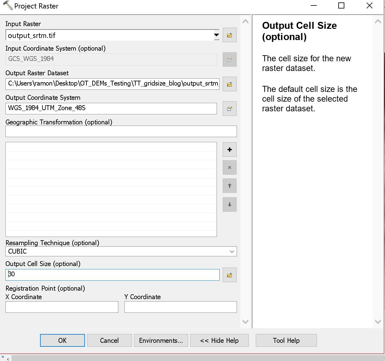
To be useful for most geomorphic analyses, the data should be projected to UTM so that the horizontal and vertical units are the same. Often, the projection is done in ArcGIS. And, usually it seems fine to let Arc determine the cell size automatically.

Notice how ArcGIS decided that the resolution for the cells should be: 30.8462728281739.

Here I set the cell size to exactly 30 m

Turning to TopoToolbox, as we compute drainage network properties, including contributing area, there is a check that the cell sizes are the same (inside the GRIDobj.m function):

if abs(abs(dx)-abs(dy))>1e-9;
    error('TopoToolbox:GRIDobj',...
    'The resolution in x- and y-direction must be the same');
    end

The 1e-9 is a somewhat arbitrarily small number which one would think would not cause a problem.

I looked into this problem tracking along with the TopoToolbox processing and some of the MATLAB built in tools.

1. Read the geotiff using MATLAB's geotiffread:

   [demdata, R] = geotiffread(filename);
   geotiffreaddifference = R.CellExtentInWorldX-R.CellExtentInWorldY;
   

   The R object has a number of values including the cell size of the geotiff:
   

   R.CellExtentInWorldX= 30.79776426908749800
   R.CellExtentInWorldY= 30.79776426908791000
   R.CellExtentInWorldX-R.CellExtentInWorldY= -4.12115e-13
   

2. Read the geotiff into the DEM object in TopoToolbox and do a similar check as above (refmat is similar to R):
   

   DEM = GRIDobj(filename);
   refmatdifference = abs(DEM.refmat(2,1))-abs(DEM.refmat(1,2));
   

   Again we see the same very small grid size difference:
   

   abs(DEM.refmat(2,1))-abs(DEM.refmat(1,2))= -4.12115e-13
   

3. The problem comes in a calculation that builds out the x and y vectors that includes a cumulative multiplication from the grid sizes inside a TopoToolbox function refmat2XY:
   

   nrrows = siz(1);
   nrcols = siz(2);
   
   x = [ones(nrcols,1) (1:nrcols)' ones(nrcols,1)]*R;
   x = x(:,1)';
   
   y = [(1:nrrows)' ones(nrrows,2)]*R;
   y = y(:,2);
   

   R is the refmat object. But, here we get the error:
   

   dx=x(1)-x(2)= -30.79776426916942000
   dy=y(1)-y(2)= 30.79776426777243600
   abs(dx)-abs(dy)= 1.39698e-09
   

   Which then would fail the GRIDobj test.
If I run the same set of checks on the file I projected with exactly 30 m grid cell size (recall above), I don't get the problem:


geotiffread:
R.CellExtentInWorldX= 30.00000000000000000
R.CellExtentInWorldY= 30.00000000000000000
R.CellExtentInWorldX-R.CellExtentInWorldY= 0
refmat difference as produced from GRIDobj:
abs(DEM.refmat(2,1))-abs(DEM.refmat(1,2))= 0
Difference after GRIDobj2mat:
dx=x(1)-x(2)= -30.00000000000000000
dy=y(1)-y(2)= 30.00000000000000000
abs(dx)-abs(dy)= 0

I think what is happening is a bit of roundoff error (see this link for detailed discussion: What Every Computer Scientist Should Know About Floating-Point Arithmetic, by David Goldberg): "Therefore the result of a floating-point calculation must often be rounded in order to fit back into its finite representation." MATLAB does all of its calculations by default in double precision, so we should have access to 16 decimal digits (e.g., https://en.wikipedia.org/wiki/IEEE_754-1985). So, why we loose precision up to 10^-9 at times is a little surprising to me, but it can obviously happen.

Thus there are a couple of workarounds:

1. Comment out the dx and dy check in GRIDobj:

   %if abs(abs(dx)-abs(dy))>1e-9;
   %    error('TopoToolbox:GRIDobj',...
   %    'The resolution in x- and y-direction must be the same');
   %    end
   

   Or make the threshold larger.
2. Explicitly set the grid resolution to a round number when projecting in ArcGIS or other software.
3. Use the reproject2utm.m command to project dems before using other TopoToolbox operations. It sets the resolution to be exactly the same for x and y

Here is a script to run these calculations: DEM_cell_size_Script.m

Thanks to Chris Crosby, Benjamin Gross, Wolfgang Schwanghart, Kelin Whipple, and Mike Zoldak for discussions.

Field trip in NW Himalaya (Himachal Pradesh)

I just returned from a very interesting and pleasant field trip in Himachal Pradesh (India) to examine the major elements of the frontal portion of the NW Himalaya. The trip was lead by Dr. Rasmus Thiede of the University of Potsdam (UP). This was my third trip to the Himalayas (the first in 2001 to the Sutlej and Spiti Rivers with UP colleagues including Rasmus and Bodo Bookhagen when they were starting their Ph.D.s under the supervision of Professor Manfred Strecker; the second was in 2010 with Dr. Wendy Bohon in the Ladakh region to contribute to her work along the Karakoram Fault in the Pangong Range area). We joined two UP students (Katharina Kretzschmar and Markus Nennewitz) who had been working in the area for two weeks already, focusing on developing a structural profile across the principal faults of the NW Himalaya in the region. I overlapped for a day with Dr. Saptarshi Dey who worked on his Ph.D. with Rasmus in the Kangra reentrant (see Dey, et al., 2016a,b). And, it was a pleasure to meet Professor Vikrant Jain from IIT Gandhinagar and his Ph.D. students. I did not (yet) get their last names but they were Ramindran, Sonam, and Pritha. Tashi Gyatseo is a long-time guide and friend of Rasmus who was chief of logistics for the trip. It was fun to meet everyone and to discuss the geology and geomorphology as well as learn a bit more of eachother's cultures.

Along with strengthening the collaborations among the groups, there were a couple of scientific targets of the trip. They build to a large degree from the Ph.D. work of Saptarshi Dey and focus on:

1. The role of climate modulation of the sediment supply and transport capacity along the major river systems and the development (and removal) of fluvial fills and terraces.
2. The activity of the major faults of the system, including the Himalayan Frontal Thrust and out of sequence faulting (activity higher in the tectonic wedge) possibly influenced by load variation from changes in sediment storage in the orogenic wedge.

So, we looked at a lot of interesting fluvial terraces mostly along the Ravi River system as well as reviewed the major structural elements of the system: HFT, Siwaliks, Main Boundary Thrust (MBT), and the Main Central Thrust (MCT).

Overview figure of the region from Gavillot, et al., 2016. The box shows the location of our trip and the map shown below.

Overview of the field trip with the orange-red line showing most of our tracks and the yellow points my main obversation locations. I am using the GaiaGPS app for my mapping. It seems ok but I might look for a more geologically oriented app for the next trip.

Panorama and annotated overlay showing the major structures and bounded rock units

Pictures

View of the nice mountains (Dhaula Dhar Range) from the Kangra airport--a nice way to start the trip!

Katharina, Markus, and Rasmus with the impressive Dhaula Dhar Range behind as seen from the Kangra area.

Most of the group at a stop along the Main Boundary Thrust where a spring may indicate increased permeability along the fault zone (yellow-white material at left is travertine).

Upper Siwaliks at sunset

Katharina in the MCT mylonites.

Chambo Town--built on an important probably 10 ka terrace. We spent a pleasant cool night there.

Pretty agricultural terraces on a high terrace south of Chamba.

Nice terraces near the Chemera Reservoir.

Stair step terraces in a tributary a few km below the Chemera Reservoir.

Rasmus is a great teacher and it was wonderful to learn from him. Here he is near some fine grained schists discussing their reflection of the overall deformation in the MCT zone.

References cited
Dey, S., Thiede, R., Schildgen, T., Wittmann, H., Bookhagen, B., Scherler, D., and Strecker, M. Holocene internal shortening within northwest Sub-Himalaya: Out-of-sequence faulting of the Jwalamukhi Thrust, India: Tectonics, 2016a.

Dey, S., Thiede, R. C., Schildgen, T. F., Wittmann, H., Bookhagen, B., Scherler, D., … Strecker, M. R. (2016b). Climate-driven sediment aggradation and incision since the late Pleistocene in the NW Himalaya, India. Earth and Planetary Science Letters, 449, 321–331. https://doi.org/10.1016/j.epsl.2016.05.050

Gavillot, Y., Meigs, A., Yule, D., Heermance, R., Rittenour, T., Madugo, C., & Malik, M. (2016). Shortening rate and Holocene surface rupture on the Riasi fault system in the Kashmir Himalaya: Active thrusting within the Northwest Himalayan orogenic wedge. Bulletin of the Geological Society of America, 128(7), 1070–1094. https://doi.org/10.1130/B31281.1

Landers earthquake fault scarp Structure from motion

I made a movie of structure from motion high resolution view of 1992 Landers California earthquake fault scarp. Video starts with 2012 hillshade (Johnson, et al., 2014; available from OpenTopography here: link) in Google Earth to show location and then to a ground based set of photographs (see blue rectangles as focal planes) visualized in Agisoft Photoscan.

I am pretty pleased that the ground-based model worked so well. Now we can move forward with fine scale alignment with earlier topographic point clouds and compute differences over the 25 years since the earthquake--a project I have worked on with Dallas Rhodes for many years (see Arrowsmith and Rhodes, 1994 and also Haddad, et al., 2012).

See also these posts:

2015 Anniversary of 1992 Landers California earthquake

SfM mapping--also has an orthophoto kmz of the Johnson, et al., 2014 data

Structure from Motion micro documentary from Merri Lisa Trigilio

References:

• Arrowsmith, J. R., & Rhodes, D. D. (1994). Original forms and initial modifications of the Galway Lake Road scarp formed along the Emerson Fault during the 28 June 1992 Landers, California, earthquake. Bulletin - Seismological Society of America, 84.
• Haddad, D. E., Akciz, S. O., Arrowsmith, J. R., Rhodes, D. D., Oldow, J. S., Zielke, O., … Shilpakar, P. (2012). Applications of airborne and terrestrial laser scanning to paleoseismology. Geosphere, 8(4). https://doi.org/10.1130/GES00701.1
• Johnson, K., Nissen, E., Saripalli, S., Arrowsmith, J. R., McGarey, P., Scharer, K., … Blisniuk, K. (2014). Rapid mapping of ultrafine fault zone topography with structure from motion. Geosphere, 10(5). https://doi.org/10.1130/GES01017.1

New report: NASA Challenges and Opportunities for Research in Earth Surface and Interiors

The new report: NASA Challenges and Opportunities for Research in Earth Surface and Interiors has just been released officially. The main link to download is here: PDF.

I was honored to be on the writing team and contributed to the surface process, human activities, topography, increasingly interconnected world, and professional development portions. We were charged with revisiting and updating the 2002 Solid Earth Science Working Group report “Living on a Restless Planet” (the SESWG Report). The update follows the SESWG framework and updates on many of the science and technology topics and will help to chart NASA Earth Sciences and Interiors priorities.

Thanks to the rest of the committee, our co chairs James Davis and Louise Kellogg, and Ben Phillips from NASA.

Accumulating links and interpretation for earthquake M7.8 - 53km NNE of Amberley, New Zealand

I am accumulating some links and thoughts with respect to today's earthquake M7.8 - 53km NNE of Amberley, New Zealand. I hope that the damage won't be too severe and I am sending positive energy to the people there. Magnitude and depth were increasing as the seismologists reviewed the seismograms. It was felt widely across New Zealand (Felt reports:

>15,000 felt reports as of 17:14 UTC

Here is a sketch of the NZ tectonic setting (from https://twitter.com/stef92320):

March 6, 2017 update:
GNS updates including offshore faulting from high resolution bathymetry

Jan. 1-4 updates:
GNS field work blog
New Zealand Geographic article
Before and after images

Dec. 5 updates:
Kekerengu Fault field work blog

Nov. 28 updates:
Kekerengu Fault and prior trenching (GNS)

Nov. 27 updates:
Repeat satellite imagery showing big shift! (Chris Milliner)
Geospatial Information Authority of Japan interesting differencing
EarthJay blog post

Nov. 25 updates:
Farm track ruptured by fault drone video
The Kekerengu Fault rupture pictures from Julian's Rock and Ice Blog

Nov. 23 updates:
NPR report with some of the amazing drone videos and other commentary
Temblor site with some of the amazing drone videos and other commentary

Nov. 21 updates:
Amazing drone video of the Kekerengu Fault rupture
Kaikora coastal uplift
Skateboarders making the most of the rupture....
Rob Langridge GNS Science talks earthquakes with JR

Nov. 19 updates:

GeoNET: viewing the earthquake from space
GeoNET: measuring the earthquake with GPS
Fagereng, Complex Earthquake Raises Complex Questions (EOS)
Trembling Earth blog entry 2

Nov. 17 updates:
Evolving magnitudes on quakestories
Preliminary landslide mapping

Nov. 15 and 16 updates:
GNS Blog
Trembling Earth blog entry 1
COMET for interferogram and interpretation
Kaikoura district faults report by GNS
Temblor interpretation
Commentary in Spinoff--GNS scientists interviewed
Science commentary
Duffy and Quigley commentary in the Conversation
Tsunami damage Banks Peninsula
Digital Globe images of surface rupture from Ryan Gold (USGS)
Preliminary Sentinel-1 interferogram
Yahoo News Seafloor uplift article

Nov. 14 updates:
Geonet what we know so far
Geonet update
IRIS Recent Earthquake Teachable moment
IRIS Special Event Site: South Island, New Zealand
Surface rupture, landslides, damage:

• Amazing surface rupture (latter portion of video)
• AGU Landslide blog entry
• Alex Perrottet tweet
• Video of rupture through house
• NZ Herald video

Nov. 13 Interpretion: The magnitude and depth (as long as it does not get much deeper) could be consistent with a rupture on the Hope Fault. The location and to some degree the focal mechanism would be more consistent with one of the thrust faults further to the west. As information has flowed in, I get a sense that the rupture was deeper and mostly underneath the main crustal faults and approaching the subduction interface below.

Reports are coming in that there is a tsunami that was generated and has hit the coast with heights of a few meters in places.

Interesting to see aftershocks aligned along the faults to the northeast. USGS tectonic summary suggested some slip along the megathrust. I wonder if it is in a sort of accretionary complex above the megathrust and transitioning into to the shearing plate boundary (hence the depth and steeper dip and oblique slip focal mechanism). USGS finite fault and source time function show deeper slip almost 100 km northeast (and 60 seconds) from the hypocenter (making this a complex earthquake). Peak slip is ~ 4m (oblique) at about 25 km down dip distance from the surface along a 38 degree to the NW dipping surface. See also IRIS backprojection results. But that is necessarily a simple model. The Cape Campbell GPS station moved 2 m E, 1 m N, and 1 m up apparently (scroll down) and that would imply shallower or greater or more complex slip than the simple inversion implies. It makes me wonder what surface rupture will look like. USGS finite fault source now indicates strong ground motions and likely seafloor uplift zone (Kaikora to almost Wellington; see the image below).

Here is a mashup of GNS faults with the USGS location, shaking estimates, additional earthquakes, and focal mechanism as of 16:23 UTC:

Links (some coming from twitter feed)

• #eqnz tweets and some on #nzeq
• NZ Civil Defence Twitter
• GNS site for the event
• GNS blog entry
• USGS site for the event--See tectonic summary and finite fault
• USGS EQ Summary poster
• Tide gages--look at ones in NZ
• Wellington tide gauge
• Castle Point tide gage
• IRIS assets on the event
• GNS active faults database
• GEOFON Potsdam GFZ page
• Locally generated tsunami along the Kaikoura coastal margin: Part 1. Fault ruptures, Walters, et al., 2010--paper with a nice map of faults in the area and information about tsunamigenic sources

News links:

• Radio NZ live updates
• Stuff live feed
• News hub feed
• NZ Herald briefing
• Stuff NZ item
• New York Times item
• BBC item

Introduction to Structure from Motion (SfM) Photogrammetry for Earth Science Research and Education short course (Sept. 24, 2016 at the GSA meeting)

Chris Crosby (UNAVCO), Ed Nissen (Colorado School of Mines), and I recently ran a one day short course at the Geological Society of America Meeting on an Introduction to Structure from Motion (SfM) Photogrammetry for Earth Science Research and Education. We had a good time sharing our enthusiasm for Structure from Motion with the group of 25 or so enthusastic participants. They came from a range of backgrounds as educators as well as researchers in active faulting, geomorphology, sedimentary geology, engineering, and more.

The course web site has some very useful content lectures and exercises. And, Chris reminded us of some quite helpful SfM docmentation that he and Katherine Shervais put together:

• Structure from Motion (SfM) Introductory Guide
• Structure from Motion (SfM) Agisoft PhotoScan processing guide

The workshop was co-sponsored by UNAVCO as well as OpenTopography. At OpenTopography, we are staring to provide SfM data and are working to build a drag and drop capability for user contributed correctly documented SfM datasets.

Ed Nissen giving the Introduction to Structure from Motion

COMET Topography Workshop 31/3/2016 – 1/4/2016

The COMET Topography workshop just completed (31/3/2016 – 1/4/2016) with great success. It was hosted by the Oxford University Earth Sciences and ably lead by Austin Elliott (also active here: @TTremblingEarth). John Elliott, David Mackenzie, and Zhou Yu made important contributions. Professors Barry Parsons and Rich Walker provided oversight. I had a great time helping out with the workshop. It was great fun to share our enthusiasm for high resolution topography and to represent and present OpenTopography to the esteemed group of mostly earthquake faulting and volcano scientists.

The workshop emphasized topography produced from photogrammetric methods. The first emphasis was on more traditional photogrammetry applied to relatively high resolution space-based bi- or tri-stereo imaging (e.g., SPOT and Pleiades). The software of choice was ERDAS Imagine with its Photogrammetry Suite. I enjoyed learning more about this technology and these data which the Oxford team among others has been using with great success for characterizing active faulting.The second emphasis was on Structure from Motion--something I have some more experience with. It was great to see the strong interest and burgeoning expertise among the various participants as they apply this methodology with ground and UAV-based images to a range of faulting and volcanic problems. The OpenTopography workshops over the last couple of years have featured SfM as well (with great contributions from Ed Nissen). I got a good primer on georeferencing and networked SfM.

The workshop agenda is here: link.

See also this nice blog post about the workshop: link.

The group photo. Sunny moment in Oxford; lots of great scientific power here and a fun lot too! Photo by David Sandwell (Oxford University).

Introductory science motivations: "Sharpening our view of earth processes with high resolution topography". Photo by David Sandwell (Oxford University).

Short Course just completed: Imaging and Analyzing Southern California's Active Faults with High Resolution Topography

We just completed our most recent OpenTopography short course: Imaging and Analyzing Southern California's Active Faults with High Resolution Topography. The course was sponsored by The Southern California Earthquake Center, UNAVCO, EarthScope, and OpenTopography. It was a pleasure to work again Chris Crosby and Ed Nissen and many thanks to Alana Williams (along with Jessica Sutton, Barrett Salisbury, and Gayatri Marliyani) for the local logistical support.

Nice montage put together by Barrett Salisbury for the course advertisement.

We had 90 applications for just 34 slots, so we emphasized early career scientists (mostly graduate students), and research in Southern California given SCEC's sponsorship. We hope to run another course soon (April 2016?) to catch up a bit more with the demand. It was wonderful to meet new people and share our enthusiasm for high resolution topography!

Students hard at work in the computer lab--Ed Nissen at the controls.

New: We recorded some of the talks. I made a summary playlist of my talk as a test. The audio is not great, but it is a summary motivation for the meeting: Sharpening our view of earth processes with high resolution topography

Summary write up for EarthScope newsletter but of relevance here too:

High resolution topographic data has become an important tool for earthquake scientists to make detailed observations and model surface evolution. Within the last decade, several efforts have been made to collect high resolution topographic (HRT) data for active faults (e.g. The B4 project, EarthScope, and numerous National Center for Airborne Laser Mapping--NCALM and USGS projects). These datasets are freely available online through OpenTopography, a NSF funded data distribution portal. The active faulting community has taken great interest in these exciting datasets, using them to generate new and important insights into earthquake processes in Southern California and elsewhere.

The EarthScope program supported the acquisition of several thousand square km of high resolution topography from lidar along active faults of the western US. The target areas included Northern, Southern & Eastern California (everything not already covered by the B4 project along the San Jacinto fault and southern San Andreas Fault; Prentice, et al., 2009), Yakima (Washington), Alaska (portions of the Denali rupture and Totschunda fault--see figure), and the Intermountain Seismic Belt (portions of the Wasatch Fault and Yellowstone). These data have been invaluable for studying deformation processes in a complementary mode to the fault zone drilling, geodetic, and seismological observatories of EarthScope.

Reference:
Prentice, C. S., Crosby, C. J., Whitehill, C. S., Arrowsmith, J R., Furlong, K. P., Phillips, D. A., GeoEarthScope LiDAR illuminates northern California's active faults, EOS Transactions of the American Geophysical Union, v. 90, no. 7, p. 55, 2009.