I tried to combine some ideas building from our OpenTopography project with nascent ML collaborations with Dr. Zhiang Chen. Thanks for their contributions.
Opportunities associated with AI/ML are really exciting, but there is a lot to think about for infrastructure, research, and education.
Our OpenTopography project was honored at this year's AGU with the Open Science Recognition prize: "For outstanding contributions in cyberinfrastructure, data management, training, and outreach associated with open-access high-resolution topography." It is a great honor and nice reognition for more than 15 years of work by our team. Huge thanks to Roman DiBiase for leading the nomination and for the letter writers Mike Oskin, Paola Passalacqua, and Josh Roering.
Chelsea Scott and Chris Crosby made a nice presentation summarizing our efforts. The recording is here: link.
It was also nice to meet the other winner, Tasha Snow and appreciate her efforts. In particular, I really appreciated her articulation of Open Science values (image from her presentation):
Our geoscience courses have benefited from plenty of course development, especially lately as we have moved online and virtual. I recently was able to invest SESE course fees to build out our capabilities for high resolution mapping and 3D work. Javier Colunga built a nice and fast Windows workstation, and we also purchased a Mavic Pro 2 sUAS system. The descriptions are below for reference.
Workstation description
We have been building these "gaming" style fast desktops for a while and this latest incarnation is powerful for graphics intensive and 3D work, especially structure from motion photogrammetry (e.g., Johnson, et al., 2014 and GSA short course).
Here is a short description of the hardware (cost approx. $5k):
CPU: Ryzen Threadripper 3970X 32-core/64-thread (with a premium cpu cooling solution)
Main Memory: 128GB DDR4 3600
Graphics Card: GeForce RTX 2080 Super
Storage: Samsung 1TB M.2 NVME OS drive, additional 4TB hard drive
Operating system: windows 10 Enterprise
Input: Logitech wireless keyboard and mouse
Monitor: HP 27 inch 1440P
Here is the main software installed:
Google Earth Pro
Matlab R2020a
Camtasia 2020
Cloudcompare
Agisoft Metashape
ArcGIS 10.7
QGIS
Here is more description, how to connect remotely, and a sign up sheet. LINK
sUAS description
For SESE, we have purchased a DJI Mavic 2 Pro (actually the FlyMore combo so it has a nice case and 3 batteries). This is a nice mapping and aerial documentation system.
Devin Keating has been helping to get the system into production mode. He has built a nice documentation of the system and its use. He also registered it with the FAA so we have a tail number. See this LINK. To operate it, one should have the part 107 Remote Pilot certification. And, there are ASU oversight requirements as well.
Recent course related work using this type of system (and computed on the nice workstation described above):
We recently visited the Warford Ranch Volcano which is a low shield volcano that is part of the Sentinel-Arlington volcanic field of southwestern Arizona. It is about 3 million years old. It was a favorite field trip destination of Prof. Ronald Greeley. Shelby Cave worked on the Sentinel-Arlington field for her Ph.D. dissertation under the supervision of Prof. Greeley and after his passing she worked with Prof. Amanda Clarke.
Google maps location for Warford Ranch (NW of Gila Bend, AZ).
Professor Clarke is teaching the Advanced Field Geology course and she took the group to Warford Ranch volcano to examine its volcanology. I did some UAS-mapping to help with the documentation. This blog entry presents some of the products of the overflights with our Mavic Air and Phantom 4 Pro.
Oblique overviews
I flew the Mavic Air high to get some views over the volcano to assess its general form and the relation to adjacent landforms and geology.
View to the north. The cars are lower left are in our parking spot. LINK to jpg
Fissure zone on SW side of higher topography. People for scale. Not sure the purpose of the excavation. LINK to jpg
Masked and socially distanced field work. LINK to jpgVideo overflight.
sUAS mapping
Along with the free flying overviews, I flew in mapping mode (using the PX4D mapper app) over most of the volcano taking 1778 images in mapping mode. I processed those in Agisoft Metashape to produce a colored point cloud, digital elevation model, and orthophoto. The latter two can be the basis of more mapping in ArcMap.
Tour of the data and its processing in Agisoft Metashape and ArcMap.
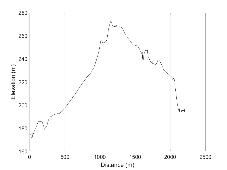
The video presented above discusses the topographic profile cut from the DEM in ArcMap towards the end. This would be the basis for the geologic cross section, preferably without vertical exaggeration.
Topographic profile location. Bent along the path of our Saturday November 22, 2020 tour. LINK to png.
Topographic data text file: LINK and MATLAB script to plot it: LINK
Even before the COVID-19 crisis changed everything, I was working this semester to build some virtual options for my Field Geology I (GLG451) course. Two students are physically unable to do the field work, and then another had a crisis and missed two weekend field trips. The course has three weekend field trips and then a mini camp over spring break.
Locations of the field trips.
I decided to try to build some digital versions of the field trips using very high resolution digital elevation models and orthophotos from our SUAS systems (thanks to Tyler Scott for doing the flying and the SfM work). I wanted these to be as similar as possible to what the regular students experience so I give some initial information on the maps as well as numerous pictures from the ground and videos from the sUAS. For most of the exercises in the case of my class, I also am providing rock samples to the students of each of the mapping units.
All of the information for each of the assignments is in a long pdf which has the text assignment, links to data and images, etc. and then some explanation. It also has a topographic profile for a cross section, etc.
I am very happy to share with anyone who might find these useful. Here are the modules and the current status:
I am organizing for a presentation to my research group on fault scarp analysis. This is an ongoing obsession of mine. I have blogged about this topic here with some review. That is still a pretty good summary of things. I also have a couple of relevant Landers Earthquake posts here and here. And, we applied many of the relevant tools to analysis of cinder cone forms.
The 2017 post mentioned above is still a pretty good summary of things. However, the MATLAB-based guis for Penck1D and Scarpdater are not running well now on newer versions of MATLAB; they need an overhaul. We were really into guis back then but they require so much code relative to the actual modeling. Might be cool to rewrite in Jupyter notebooks, maybe see how much in landlab could be used.
I have prepared a new review powerpoint (PPT and PDF) with this outline:
Introduction and review
Diffusion-equation analysis of scarplike landforms
I just returned from my second year of participation in the Specialization certificate for the assessment and management of geological and climate related risk (CERG-C) course in Geneva (Switzerland) and Vulcano Island (Sicily, Italy). It was stimulating, interesting, and beautiful. The course takes a "...multidisciplinary approach to the assessment and management of risk from natural hazards, merging ideas from disciplines such as the physical and social sciences, engineering, and economics" (website). The course has 8 modules and there were about 25 students from around the world participating. The course is lead by Professor Costanza Bonnadonna. Several other instructors participate and getting to know them has been quite nice. Amanda Clarke and I have joined the last few years
It is a tough place to work: view from La Fossa towards Vulcanello across the Vulcano town with Lipari and other Aeolian Islands behind
The last two years I have helped by providing a series of lectures in Geneva on topography and then participated in the field exercise on Vulcano Island (Sicily, Italy). I argue that it is a fundamental geophysical dataset for any hazard and risk assessment as it drives and resists processes and hazards. After all, potential energy = mass x gravity x relative height. Topography fits in the realm of Geodesy which is the science of accurately measuring and understanding three fundamental properties of the Earth: its geometric shape, its orientation in space, and its gravity field—as well as the changes of these properties with time. We know that surface processes act to change elevation through erosion and deposition while tectonic processes depress or elevate the surface directly. And, topography and geomorphology (study of landforms and surface processes) helps to link between timescales of seismology and crustal deformation (1-10 yr) and geology and tectonics (1-10 Myr)
Vulcano and topography and bathymetry of northern Sicily. Note that I demonstrate the very useful geomapapp.
I also demonstrate ArcGIS and show the data and topography from Vulcano.
At Vulcano, the students have the opportunity to put into practice their hazard and risk knowledge. The program starts with a field trip and lectures on the various volcanic hazards (unrest and degassing, single vulcanian, persistant vulcanian, subplinian from the main edifice ("La Fossa") and strombolian and lava flow eruptions from the adjacent "Vulcanello). Then the students work through vulnerability, warning messages, and even have a crisis exercise. They stay busy from 8 am to 10 pm. The studnet have to present almost every night a poster on what they analyzed for that day, with the assembled instructors as audience and evaluators. There are also evening lectures including a review of Italian earthquakes with extended lecture on L'Aquila by me and a very nice review of Italian Civil Protection by one of its representatives. And, one of the highlights is a volcano crisis "play" at the local elementary school in which the students have a script and take various roles as community members, media, safety staff, government officials, scientists, etc. to go throught a possible volcanic crisis at Vulcano. It was very cute and a great demosntration of how to engage communities to understand the hazards they face and what to do.
Professor Mauro Rosi from University of Pisa lecturing to the group with La Fossa vent behind.
Nice action video from the Mavic Air
INGV team demonstrating gas sampling from the fumaroles.
In order to demonstrate acquisition of topography as well as collect some for some of the research activities ongoing at Vulcano by the team, I worked with an INGV colleague Il maestro Dr. Fabio Pisciotta to collect photos from drones for structure from motion reconstructions. He has a lot of experience droning at Vulcano and was a great teacher. We teamed up with his Phantom 3 and our Phantom 4 Pro and collected more than 6000 images over the edifice. Stay tuned for the models...
Introduction. In my last post, I showed how I had extracted frames from satellite-derived video to build a 3D model of a mine from space. In this post, I show a similar workflow for phone camera: take a video of an object (some times a lot easier than numerous frames although lower quality) and make a 3D model using Agisoft Photoscan.
Video to images. (this part is repeated from the last post). The main generic challenge for SfM from video is to extract the video frames and prepare them for the SfM. The SfM part is no different from what my group has been doing for a while with Agisoft Photoscan. I used MATLAB to do the video processing. The script is here: readplanetvid.m. The main code bits include:
PlanetObj = VideoReader(videoname); %make a video object from an MP4 file

vidWidth = PlanetObj.Width;         %get the width

vidHeight = PlanetObj.Height;       %and height


mov = struct('cdata',zeros(vidHeight,vidWidth,3,'uint8'),...

    'colormap',[]);  %set up a MATLAB structure to contain the video


k = 1;

while hasFrame(PlanetObj)

    mov(k).cdata = readFrame(PlanetObj); %pull out the frames one at a time from the MP4 object and put them in the mov

    k = k+1;

end


step = floor(k/number_of_frames) %determine how many frames to skip each time to get the desired number

for i = 1:step:(k-1)

    framepart = sprintf('_frame_%06d.png', i);

    filename = strcat(foldername,'/',projectname,framepart);

    imwrite(mov(i).cdata, filename)  %easy to write the frame out as a png file

end
Video of a rock sample in my backyard. I took a short video of a piece of obsidian on a table with my Samsung J3. The nice thing about it was that I could gather a large number of views around the sample with relative ease. From that video, I extracted 150 frames, for example see below
I ran the files through the Agisoft Photoscan sequence of alignment (high), build dense cloud (medium), build mesh (medium), and build texture (medium). Here are a few screen captures of the result:
This one shows a somewhat complex background, but nicely indicates the path of the camera too.
And here it is with a trim to only show the sample on the table:
Video to images. The main generic challenge for SfM from video is to extract the video frames and prepare them for the SfM. The SfM part is no different from what my group has been doing for a while with Agisoft Photoscan. I used MATLAB to do the video processing. The script is here: readplanetvid.m. The main code bits include:
PlanetObj = VideoReader(videoname); %make a video object from an MP4 file

vidWidth = PlanetObj.Width;         %get the width

vidHeight = PlanetObj.Height;       %and height


mov = struct('cdata',zeros(vidHeight,vidWidth,3,'uint8'),...

    'colormap',[]);  %set up a MATLAB structure to contain the video


k = 1;

while hasFrame(PlanetObj)

    mov(k).cdata = readFrame(PlanetObj); %pull out the frames one at a time from the MP4 object and put them in the mov

    k = k+1;

end


step = floor(k/number_of_frames) %determine how many frames to skip each time to get the desired number

for i = 1:step:(k-1)

    framepart = sprintf('_frame_%06d.png', i);

    filename = strcat(foldername,'/',projectname,framepart);

    imwrite(mov(i).cdata, filename)  %easy to write the frame out as a png file

end
Satellite video from Terra Bella. I have been watching the hi resolution satellite activity with great interest. Skybox had a few relatively high res (approx 1 m ground resolution) visible and near IR satellites with video capability. They were bought by Terra Bella (google) and then now are owned by Planet (who were just visiting us on the ASU campus last week and with whom we are building some collaborations). Some of the Terra Bella imagery is available on youtube. I grabbed one video of the Usak Mine in Turkey (used real player to convert youtube to mp4):
You can really see the parallax as the satellite moves over (not to mention the activity of the vehicles).
I ran my script on the mp4 and extracted 100 png frames. Here is an example:
I ran the files through the Agisoft Photoscan sequence of alignment (high), build dense cloud (medium), build mesh (medium), and build texture (medium). Here are a few screen captures of the result:
You can see the model and the camera positions. They are in the roughly correct arc, and relatively far away, but they should be much farther (orbit is approx 450 km).
Nice looking textured mesh. It is distorted, but not too bad, all things considered!
What did we learn? We learned that the SfM from video is doable (see a future post from my backyard and phone video). Here is the Photoscan report on the Usak project. The geometry that is computed from the satellite video is not bad. Agisoft Photoscan does a pretty good job. We cannot get under the hood very easily to see more about the processing. I think that someone who knows more about computer vision than me would be able to comment as to the performance. I think that the main issue is probably the relatively low angular variation for the model.
Planet Team (2017). Planet Application Program Interface: In Space for Life on Earth. San Francisco, CA. https://api.planet.com.
Two short courses are scheduled for mid June at Potsdam University. The short courses are independent of each other; however, the topics are related and probably address a similar audience.
Geoscience investigations of point clouds, June 7-9, 2017. Instructors B. Bookhagen, R. Arrowsmith, M. Isenburg, C. Crosby.
This course will explore the acquisition, post-processing, and classification of point clouds derived from airborne and terrestrial lidar scanners and structure from motion (SfM) photogrammetry from drones. The course will take place at campus Golm (UP) and includes one day of field-data collection and two days of data post-processing and analysis.
The application is here: https://goo.gl/forms/NrRAcaASXPuseRs62. The course is sponsored by Geo-X.
Here is the flyer: PDF for more details.
Advancing understanding of geomorphology with topographic analysis emphasizing high resolution topography, June 12-15, 2017. Instructors R. Arrowsmith, W. Schwanghart, C. Crosby, B. Bookhagen.
This course will focus on advanced understanding of geomorphology with topographic analysis emphasizing high-resolution topography. The course will take place at campus Golm (UP) and includes theoretical background and analysis of digital topography using TopoToolbox in a Matlab environment. The course is sponsored by StRATEGy.
Here is the flyer: PDF for more details.
I made a movie of structure from motion high resolution view of 1992 Landers California earthquake fault scarp. Video starts with 2012 hillshade (Johnson, et al., 2014; available from OpenTopography here: link) in Google Earth to show location and then to a ground based set of photographs (see blue rectangles as focal planes) visualized in Agisoft Photoscan.
I am pretty pleased that the ground-based model worked so well. Now we can move forward with fine scale alignment with earlier topographic point clouds and compute differences over the 25 years since the earthquake--a project I have worked on with Dallas Rhodes for many years (see Arrowsmith and Rhodes, 1994 and also Haddad, et al., 2012).
Arrowsmith, J. R., & Rhodes, D. D. (1994). Original forms and initial modifications of the Galway Lake Road scarp formed along the Emerson Fault during the 28 June 1992 Landers, California, earthquake. Bulletin - Seismological Society of America, 84.
Haddad, D. E., Akciz, S. O., Arrowsmith, J. R., Rhodes, D. D., Oldow, J. S., Zielke, O., … Shilpakar, P. (2012). Applications of airborne and terrestrial laser scanning to paleoseismology. Geosphere, 8(4). https://doi.org/10.1130/GES00701.1
Johnson, K., Nissen, E., Saripalli, S., Arrowsmith, J. R., McGarey, P., Scharer, K., … Blisniuk, K. (2014). Rapid mapping of ultrafine fault zone topography with structure from motion. Geosphere, 10(5). https://doi.org/10.1130/GES01017.1
Chris Crosby (UNAVCO), Ed Nissen (Colorado School of Mines), and I recently ran a one day short course at the Geological Society of America Meeting on an Introduction to Structure from Motion (SfM) Photogrammetry for Earth Science Research and Education. We had a good time sharing our enthusiasm for Structure from Motion with the group of 25 or so enthusastic participants. They came from a range of backgrounds as educators as well as researchers in active faulting, geomorphology, sedimentary geology, engineering, and more.
The course web site has some very useful content lectures and exercises. And, Chris reminded us of some quite helpful SfM docmentation that he and Katherine Shervais put together:
The workshop was co-sponsored by UNAVCO as well as OpenTopography. At OpenTopography, we are staring to provide SfM data and are working to build a drag and drop capability for user contributed correctly documented SfM datasets.
Ed Nissen giving the Introduction to Structure from Motion
The COMET Topography workshop just completed (31/3/2016 – 1/4/2016) with great success. It was hosted by the Oxford University Earth Sciences and ably lead by Austin Elliott (also active here: @TTremblingEarth). John Elliott, David Mackenzie, and Zhou Yu made important contributions. Professors Barry Parsons and Rich Walker provided oversight. I had a great time helping out with the workshop. It was great fun to share our enthusiasm for high resolution topography and to represent and present OpenTopography to the esteemed group of mostly earthquake faulting and volcano scientists.
The workshop emphasized topography produced from photogrammetric methods. The first emphasis was on more traditional photogrammetry applied to relatively high resolution space-based bi- or tri-stereo imaging (e.g., SPOT and Pleiades). The software of choice was ERDAS Imagine with its Photogrammetry Suite. I enjoyed learning more about this technology and these data which the Oxford team among others has been using with great success for characterizing active faulting.The second emphasis was on Structure from Motion--something I have some more experience with. It was great to see the strong interest and burgeoning expertise among the various participants as they apply this methodology with ground and UAV-based images to a range of faulting and volcanic problems. The OpenTopography workshops over the last couple of years have featured SfM as well (with great contributions from Ed Nissen). I got a good primer on georeferencing and networked SfM.
See also this nice blog post about the workshop: link.
The group photo. Sunny moment in Oxford; lots of great scientific power here and a fun lot too! Photo by David Sandwell (Oxford University).
Introductory science motivations: "Sharpening our view of earth processes with high resolution topography". Photo by David Sandwell (Oxford University).
Nice montage put together by Barrett Salisbury for the course advertisement.
We had 90 applications for just 34 slots, so we emphasized early career scientists (mostly graduate students), and research in Southern California given SCEC's sponsorship. We hope to run another course soon (April 2016?) to catch up a bit more with the demand. It was wonderful to meet new people and share our enthusiasm for high resolution topography!
Students hard at work in the computer lab--Ed Nissen at the controls.
Summary write up for EarthScope newsletter but of relevance here too:
High resolution topographic data has become an important tool for earthquake scientists to make detailed observations and model surface evolution. Within the last decade, several efforts have been made to collect high resolution topographic (HRT) data for active faults (e.g. The B4 project, EarthScope, and numerous National Center for Airborne Laser Mapping--NCALM and USGS projects). These datasets are freely available online through OpenTopography, a NSF funded data distribution portal. The active faulting community has taken great interest in these exciting datasets, using them to generate new and important insights into earthquake processes in Southern California and elsewhere.
The EarthScope program supported the acquisition of several thousand square km of high resolution topography from lidar along active faults of the western US. The target areas included Northern, Southern & Eastern California (everything not already covered by the B4 project along the San Jacinto fault and southern San Andreas Fault; Prentice, et al., 2009), Yakima (Washington), Alaska (portions of the Denali rupture and Totschunda fault--see figure), and the Intermountain Seismic Belt (portions of the Wasatch Fault and Yellowstone). These data have been invaluable for studying deformation processes in a complementary mode to the fault zone drilling, geodetic, and seismological observatories of EarthScope.
Reference:
Prentice, C. S., Crosby, C. J., Whitehill, C. S., Arrowsmith, J R., Furlong, K. P., Phillips, D. A., GeoEarthScope LiDAR illuminates northern California's active faults, EOS Transactions of the American Geophysical Union, v. 90, no. 7, p. 55, 2009.
The Black Canyon City landslide (BCL) is a spectacular deep seated structure located northeast of Black Canyon City, Arizona. It does not appear to pose much harm to structures etc. but it is an interesting feature worthy of study. Such examinations are useful for understanding the geologic setting under which they develop (in this case bedded Tertiary rocks and good local relief), appreciating the potential contributions to the landscape evolution in the area with a similar setting, and for characterizing the underlying structural processes.
Figure 1. Google maps of the Black Canyon City landslide area.
I was first introduced to the BCL in the late 90s by Nick Priznar from Arizona Department of Transportation and then Phil Pearthree (Arizona Geological Survey) and I taught an Advanced Field Geology class together with one weekend focused on it. Lee Amoroso (USGS) also contributed significantly I subsequently used it in Geomorphology courses over the years (e.g., picture of group having lunch in crestal graben). Link to old pages. David Haddad worked for AZGS and contributed to mapping the quadrangle that contains the BCL: Ferguson, C.A., Haddad, D.E., Johnson, B.J., Guynn, J.H., Spencer, J.E., and Eddy, D.L., 2008,
Geologic map of the east half of the Black Canyon City 7 ½' Quadrangle and the west half of the
Squaw Creek Mesa 7 ½' Quadrangle, Maricopa and Yavapai Counties, Arizona: Arizona Geological
Survey Digital Geologic Map DGM-64, 1 sheet, scale 1:24,000, with 27 p. text.
Hurien Helmi is working with me on an M.S. degree and he has chosen to focus on the BCL which should be really great! As part of Hurien's work, we have wanted to produce high resolution maps of the BCL. Hurien has done some work with our balloon systems, but the BCL is in a fairly windy place and thus it has been a bit of a struggle to get good results. Yesterday, we went to the BCL with Professor Srikanth Saripalli our SESE colleague and flew a drone there with good results (hence the topic of this blog entry). I want to summarize the results of the Structure from Motion results from the trip. Stay tuned for Hurien's careful work. This effort is also part of a project with JPL colleagues exploring the power of structure from motion with applications to topographic mapping from space (GAZING).
Sri bought a new DJI Phantom 2 Vision Plus and we used it along with the PIX4D app running on his phone. It worked quite well in that we were able to fly for effectively 15 minutes on each of two batteries (about 10 minutes of mapping time--as indicated in the app).
Figure 2. Overview of the three missions presented as hillshades computed from 0.1 m per pixel digital surface models.
Along with the field acquisition challenge, I wanted to see the differences in results from two main pieces of Structure from Motion software: PIX4D--for which Sri has a license--and Agisoft Photoscan--with which my students and I have more experience (and for which we have a license). In this presentation, I will only show the results from Agisoft Photoscan given their cursory nature. I computed 3D models and present short videos of the texture mapped meshes from Photoscan below as well as a few screen captures. Very importantly, the 3D georeferencing only comes from the GPS tags in the original jpgs from the Phantom!. In addition, I computed digital surface models (DSM) from the models and exported 10 cm versions as geotiffs which I loaded into ArcMap and computed hillshades and cut a few topographic profiles. Aside from the topographic tilt and some other georeferencing issues, the results are impressive for a relatively low amount of effort. It seems that the software can manage the fisheye lens view from the Phantom's camera.
Mission 1 (10 minute flight 80 m above launch point): We covered the toe area of the slide in mission 1. The results are pretty good aside from a gap in the coverage.
Figure 3. Mission 1 overview. Camera positions are indicated as blue rectangles (used). The "lawnmower patter" is evident.
Figure 4. Mission 1 texture map 3D view.
3D visualization of mission 1 coverage
Mission 2 (4 minute flight 40 m above launch point): We made a small flight over the toe area where there are clear fault scarps associated with deformation of the slide (as well as significant fissuring and collapse features).
Figure 5. Mission 2 overview. Camera positions are indicated as blue rectangles.
3D visualization of mission 2 coverage
Figure 6. Toe area DSM. Topographic model shows toe scar well but the whole model has a northwestern tilt due to the simple GPS control on the images for georeferencing.
Mission 3 (11 minute flight 80 m above launch point which is only about 20 or so meters above the upper portion of the slide): We moved up to the slide body and flew over the extensional system at the head of the slide. Note some images were not used (dots in the camera locations from Photoscan)
Figure 7. Mission 3 overview. Camera positions are indicated as blue rectangles or dots (not used?).
Figure 8. 3D views over textured mesh of upper portion of slide.
3D visualization of mission 3 coverage
Figure 9. Upper portion of the slide DSM. Extensional features are quite evident with 10 m deep troughs. Georeferencing is ok.