Showing posts with label OpenTopography. Show all posts

Friday, June 5, 2026

Presentation for Harnessing Massive Data Across Geophysical Domains and Applications: Committee on Solid Earth Geophysics Spring Meeting 2026

I enjoyed the opportunity to present in the spring meeting of the National Academy of Sciences Committee on Solid Earth Geophysics Spring Meeting 2026. The meeting was entitled: Harnessing Massive Data Across Geophysical Domains and Applications.

--Photo by Wendy Bohon, PhD

PRESENTATION

I tried to combine some ideas building from our OpenTopography project with nascent ML collaborations with Dr. Zhiang Chen. Thanks for their contributions.

Opportunities associated with AI/ML are really exciting, but there is a lot to think about for infrastructure, research, and education.

San Andreas Fault in the Carrizo Plain Field trips

Recently, I pulled together some notes for the SCEC UNREST Field trip in the Carrizo Plain. It was a great conversation to share with the esteemed colleagues.


So I can find it, here are the notes that produced as a handout: LINK

Here are a few other items/guides:

Friday, December 15, 2023

Open Science recognition prize at AGU 2023

Our OpenTopography project was honored at this year's AGU with the Open Science Recognition prize: "For outstanding contributions in cyberinfrastructure, data management, training, and outreach associated with open-access high-resolution topography." It is a great honor and nice reognition for more than 15 years of work by our team. Huge thanks to Roman DiBiase for leading the nomination and for the letter writers Mike Oskin, Paola Passalacqua, and Josh Roering.

Chelsea Scott and Chris Crosby made a nice presentation summarizing our efforts. The recording is here: link.

It was also nice to meet the other winner, Tasha Snow and appreciate her efforts. In particular, I really appreciated her articulation of Open Science values (image from her presentation):

The full award ceremony is recorded here: link.

Here are a couple of pictures of our team:

Other links:
OpenTopography news release: link

And we celebrated with the other ASU / SESE awardees (Vernon Morris and Everett Shock):

Saturday, October 5, 2019

(Finally) Getting going with python (and a bit of history)

I certainly recognize the power of scientific programming. Programming spreadsheets is obvious and there is nothing to be ashamed of there (see weeks 2-6 in my Computers in Earth and Space Exploration course). I started off in grad school with Mathemematica and appreciated the notebook style of computations and integrated graphics and text. I also taught myself enough fortran to get the main calculations for my dissertation completed.


Modeling profile development with simple diffusion (Arrowsmith, et al., 1998) using fortran code and Mathematica for the basic graphics.

I took some programming courses (Pascal) back in grad school. I was not very good at it. Once the professor even said "that is the stupidest way I have ever seen for doing that" in office hours. I was not too offended; I barely understood what I was doing. Nevertheless, I got the big picture and have stumbled along ever since.

Professor George Hilley taught me many things. One thing he was able to do after a fair amount of cajoling was to get me to start in MATLAB. The more data-oriented and matrix handling of MATLAB ended being something I could use effectively. We also worked with Don Ragan a lot on MATLAB and Latex. While I am no expert, I have taught the basics to students over the years see weeks 6-9 in my Computers in Earth and Space Exploration course). I cannot say that I have had any really great programming projects, but the various analysis and plotting needs have been satisfied. For what it is worth, I even set up a GitHub page to hold a few things. Dr. Olaf Zielke is a serious MATLAB programmer and wrote some impressive tools with GUIS for his PhD and related work. TopoToolbox is another set of MATLAB-based tools which I had the opportunity to learn and appreciate their transformative power for a lot of geomorphic analyses.

I have been watching the progressive adoption of Python and related tools in my little scientific bubble over the last 5 or so years. I have not had the time to do much as far as learning until recently, however. While my MATLAB expertise won't go away, I have appreciated the fact that it is hard to share and teach with students and colleagues who don't have access to the rather expensive licenses for MATLAB. On the other hand, Python and related tools are open and apparently so adaptable and customizeable.

Recently, I finally had an excuse and the time to get my feet wet with Python. Chris Crosby and I (OpenTopography) helped out with a short course From point clouds and full-waveform data to DEM analysis (Sep-30 to Oct-4 2019) led by Professor Bodo Bookhagen and his team.


Specific catchment area computed with the tools from Rheiwalt, et al., 2019. The basic processing was in Python with some c code and then visualized using Displaz.

Here is some basic full waveform lidar processing from Bookhagen and Rheinwalt again basic procesing in Python and then visualized using Displaz.

I still don't understand all that I am doing, but I got the basic set up and can sort of understand packages and environments. Javier Colunga helped me by getting Ananconda installed. Spyder is the development environment I had been looking for. There is so much that is possible; it is hard to even know where to start.

For my first project, I thought it would be nice to play around with a lidar point cloud (using the Dragon's Back of course): grid it using pdal and then make a hillshade using gdal. Download the data from OpenTopography.

The steps are:

  1. Launch an Ananconda terminal.
  2. Add these conda channels for package install:
    conda config --prepend channels conda-forge/label/dev
    conda config --prepend channels conda-forge
  3. Then define an environment and add the packages using conda: conda create -y -n PC_py3 python=3.6 pip scipy pandas numpy matplotlib scikit-image gdal pdal xarray packaging ipython multiprocess h5py lastools pykdtree spyder gmt=5* (this comes from the workshop).

My first problem was that I could not run pdal from inside a python script. There is something I don't understand there (even though it is installed, etc.). I see that it is possible to call python from inside the pdal json files... But, I can run it from the command line:
> pdal pipeline db.json
where the db.json has the parameters for the simple neighborhood gridding run:


{
        "pipeline":[
        "smallpiece.laz",
        {
                "resolution": 1,
                "radius": 0.707,
                "gdaldriver": "GTiff",
                "gdalopts": "COMPRESS=DEFLATE, ZLEVEL=7, GDAL_NUM_THREADS=ALL CPUS",
                "data_type": "float",
                "output_type": "idw",
                "filename":"small_idw_1m.tif"
        }
        ]
}
I was able to make a little dem (the tif file). But then, I ran the gdal from the command line only:
>gdaldem hillshade small_idw_1m.tif small_idw_1m_shd.tif

Finally, I could run a little python script to draw the hillshaded geotiff (this I could run from Spyder):


#!/usr/bin/env python
import gdal
import matplotlib.pyplot as plt

ds = gdal.Open('small_idw_1m_shd.tif').ReadAsArray()

plt.close('all')

plt.imshow(ds, cmap='gray')

f.savefig('smallDB.png', dpi=300)
plt.close('all')


Small piece of the Dragon's Back lidar data (B4 project) gridded with pdal, hillshaded with gdal, and drawn with matplotlib

So, I guess that is a bit of a success, there is a lot more to do and learn!

I keep finding references to help learn:

Sunday, March 17, 2019

From crashing kites and Frankenmodels to efficient large-scale UAV acquisitions and beautiful shared 3D models (2018 GSA talk)

I was invited to give a presentation in a session at the Fall 2018 Geological Society of America session T60. Revolutions in Remote Sensing: Applications of UAVs to Field Mapping and Surface Analytics (organized by Dylan Blumentritt--Winona State University and Toby Dogwiler--Missouri State University). I decided to make a my presentation a bit of a reflection of how my own obsession with low altitude imaging had evolved and how far we had come. After all, I started in college working in the Fairchild Aerial Photography Collection when it was at Whittier College. So, I came up with a talk with the hopefully entertaining title of FROM CRASHING KITES AND FRANKENMODELS TO EFFICIENT LARGE-SCALE UAV ACQUISITIONS AND BEAUTIFUL SHARED 3D MODELS. I am putting links to the talks on line in case they might be useful: PPT and PDF.

The presentation shows a couple of maybe interesting things:

  1. It shows a pretty 3D point cloud (video above) from our Photogrammetric model of the Tecolote Volcano, Sonora, Mexico hosted at https://opentopography.org/.
  2. It spends some time talking about and making the case for the OpenTopography Community Dataspace.
  3. As part of the OpenTopography Community Dataspace discussion, I (with slides and ideas from Chris Crosby) talked about standardizing metadata for these long tail data. See for example the different styles of metadata documents ("Survey Report"): for example Almaty range front fault, Koram site or Clear Creek, Idaho post-fire debris flow erosion--note the ones I uploaded are not great examples :).
  4. Of course, one of the really nice things that the OpenTopography Community Dataspace publishing of one's data allows is to mint a DOI. That DOI allows then for a data citation. I have added a new part of my CV that has a section on data publication. Here is an example citation style:
    Arrowsmith, J R., DiMaggio, E. N., Garello, G. I., Villmoare, B. and LediGeraru Research Project (2018): Photogrammetric model of a portion of the LeeAdoyta Basin, Afar, Ethiopia (point cloud [122M points], orthophoto [2cm/pix], and DEM [25 cm/pix]). Distributed by OpenTopography. AccessedOctober 23, 2018. https://doi.org/10.5069/G95X271W.

The conclusions are useful to highlight as well:

  • We are part of a revolution in 3 and 4 D data collection and analysis
  • Additional needs for the community include
    • Optimized data acquisition strategies
    • Low cost and high performance computation of point clouds and models
    • Efficient and accurate georeferencing
    • High quality differencing for change detection
    • Bring the tools and data into the (outdoor) classroom; need more curriculum (c.f. GETSI - GEodesy Tools for Societal Issues (UNAVCO) at https://serc.carleton.edu/getsi/)
  • OpenTopography Community Dataspace
    • Great opportunity to expand the impact of emerging topography through improved access
    • Services and existing community of users
    • Community engagement & best practices
    • Please join us and start sharing your models and ideas for how to improve

Monday, June 5, 2017

Some new San Andreas Fault tour videos of 1 m bare earth hillshades

I have been preparing a lecture and I built some new simple videos flying along the San Andreas Fault. The videos are made by me flying along in Google Earth with 1 m hillshades produced from lidar topography data collected along the San Andreas Fault. The videos are on youtube in this play list: https://www.youtube.com/playlist?list=PLFfZSFyNZ_jZm86F1TsnYfuuYNef_Uh21. I also put the MP4s in this folder--they are numbered 1-8 from NW-SE.

The flights follow generally along the San Andreas Fault from Point Arena to the southern Carrizo Plain (Dragon's Back and Northern Elkhorn Hills):

The data were processed at www.opentopography.org and come from 3 really cool datasets:

Friday, May 5, 2017

Simple Topography Lectures at University of Geneva as part of CERG-C

I am visiting the University of Geneva as part of the CERG-C project. Professor Costanza Bonadonna is the leader of the activity which is a course on hazard and risk with an international group of students. They have been in Geneva for a few weeks for classroom work and starting tomorrow they go to Vulcano Island for practical experience. I am going to join.

I gave a lecture and a practical demonstration on the general topic of Topography, but trying to emphasize its fundamental value for science and applied value for hazard assessment. And, of course making the point that high resolution data are most useful.

Here are the pdfs to my lectures and demo:

Saturday, April 8, 2017

A pair of short courses on "Geoscience Investigations of Point Clouds" and "Advancing understanding of geomorphology with topographic analysis": mid June, 2017 at Potsdam University, Golm

Two short courses are scheduled for mid June at Potsdam University. The short courses are independent of each other; however, the topics are related and probably address a similar audience.

Geoscience investigations of point clouds, June 7-9, 2017. Instructors B. Bookhagen, R. Arrowsmith, M. Isenburg, C. Crosby.
This course will explore the acquisition, post-processing, and classification of point clouds derived from airborne and terrestrial lidar scanners and structure from motion (SfM) photogrammetry from drones. The course will take place at campus Golm (UP) and includes one day of field-data collection and two days of data post-processing and analysis.
The application is here: https://goo.gl/forms/NrRAcaASXPuseRs62. The course is sponsored by Geo-X.
Here is the flyer: PDF for more details.

Advancing understanding of geomorphology with topographic analysis emphasizing high resolution topography, June 12-15, 2017. Instructors R. Arrowsmith, W. Schwanghart, C. Crosby, B. Bookhagen.
This course will focus on advanced understanding of geomorphology with topographic analysis emphasizing high-resolution topography. The course will take place at campus Golm (UP) and includes theoretical background and analysis of digital topography using TopoToolbox in a Matlab environment. The course is sponsored by StRATEGy.
Here is the flyer: PDF for more details.

Thursday, March 16, 2017

Mapping landforms with applications to geomorphology and earthquake geology EXERCISE

I wanted to share a project I have developed on and off for about 10 years. It is a classroom exercise for Mapping landforms with applications to geomorphology and earthquake geology. So far, it has an example for strike-slip faults (Wallace Creek along the San Andreas Fault), and blind thrust faults (Wheeler Ridge in Southern California). I have an intention to add a normal fault example but have not finished it yet.

The basic idea is that the exercises could be done "analog"--that is on paper in a classroom. They emphasize some simple morphologic and geomorphic mapping (but on high resolution topography base maps from lidar data collected by NCALM and available for download from OpenTopography), and then provide landform ages so that students can calculate slip rate or surface uplift rates. I am not sure they are so well explained so any feed back is welcome.

Exercise material:

Sunday, March 12, 2017

DEM grid size specification and learning a bit of TopoToolbox

I have been wanting to learn TopoToolbox for a while, and last week I had a chance to get started. Spending time at the Universität Potsdam, Institut für Erd- und Umweltwissenschaften, I have met with Wolfgang Schwanghart and Dirk Scherler occasionally. They are coauthors of TopoToolbox.

My ASU colleagues Adam Forte and Kelin Whipple have been using TopoToolbox increasingly over the last few years. Recently Kelin had a question as to why some DEMs grids were causing an error in TopoToolbox and why some were not. I dug into it and here is what I found. Projected DEMs should have EXACTLY the same x and y cell sizes and expressed in precise values (nearest meter or 10th or 100th of a meter).


DEMs (such as SRTM 30 meter) can be downloaded as geotiff formats and with geographic coordinate systems from sources such as OpenTopography: select Global Data tab.


For example, I have chosen a piece of data from Java along the Cimandiri fault (see Marliyani, et al., 2016 for example).

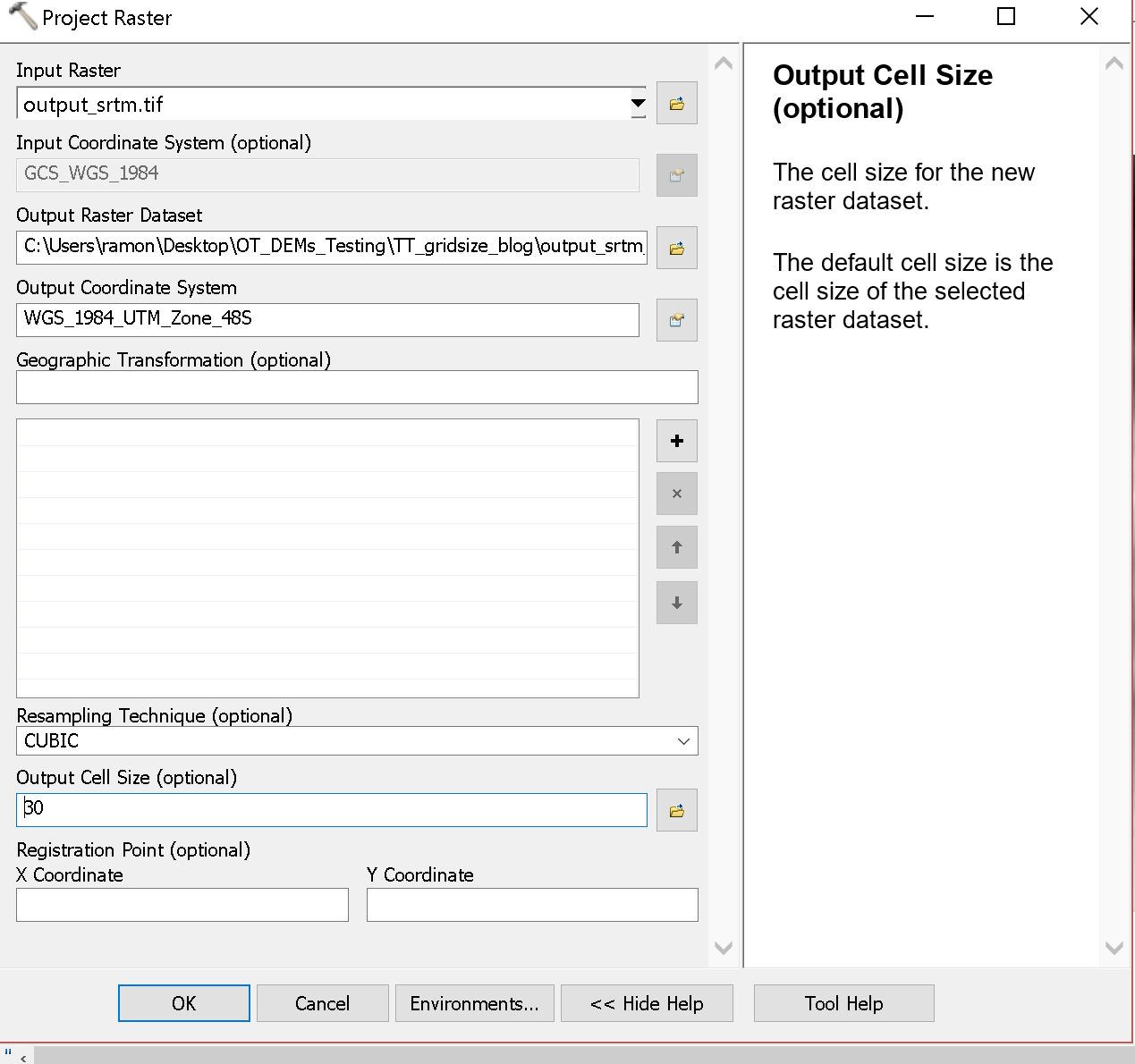
To be useful for most geomorphic analyses, the data should be projected to UTM so that the horizontal and vertical units are the same. Often, the projection is done in ArcGIS. And, usually it seems fine to let Arc determine the cell size automatically.

Notice how ArcGIS decided that the resolution for the cells should be: 30.8462728281739.
Here I set the cell size to exactly 30 m

Turning to TopoToolbox, as we compute drainage network properties, including contributing area, there is a check that the cell sizes are the same (inside the GRIDobj.m function):

if abs(abs(dx)-abs(dy))>1e-9;
    error('TopoToolbox:GRIDobj',...
    'The resolution in x- and y-direction must be the same');
    end
The 1e-9 is a somewhat arbitrarily small number which one would think would not cause a problem.

I looked into this problem tracking along with the TopoToolbox processing and some of the MATLAB built in tools.

  1. Read the geotiff using MATLAB's geotiffread:
    [demdata, R] = geotiffread(filename);
    geotiffreaddifference = R.CellExtentInWorldX-R.CellExtentInWorldY;
    
    The R object has a number of values including the cell size of the geotiff:
    R.CellExtentInWorldX= 30.79776426908749800
    R.CellExtentInWorldY= 30.79776426908791000
    R.CellExtentInWorldX-R.CellExtentInWorldY= -4.12115e-13
    
  2. Read the geotiff into the DEM object in TopoToolbox and do a similar check as above (refmat is similar to R):
    DEM = GRIDobj(filename);
    refmatdifference = abs(DEM.refmat(2,1))-abs(DEM.refmat(1,2));
    
    Again we see the same very small grid size difference:
    abs(DEM.refmat(2,1))-abs(DEM.refmat(1,2))= -4.12115e-13
    
  3. The problem comes in a calculation that builds out the x and y vectors that includes a cumulative multiplication from the grid sizes inside a TopoToolbox function refmat2XY:
    nrrows = siz(1);
    nrcols = siz(2);
    
    x = [ones(nrcols,1) (1:nrcols)' ones(nrcols,1)]*R;
    x = x(:,1)';
    
    y = [(1:nrrows)' ones(nrrows,2)]*R;
    y = y(:,2);
    
    R is the refmat object. But, here we get the error:
    dx=x(1)-x(2)= -30.79776426916942000
    dy=y(1)-y(2)= 30.79776426777243600
    abs(dx)-abs(dy)= 1.39698e-09
    
    Which then would fail the GRIDobj test.
  4. If I run the same set of checks on the file I projected with exactly 30 m grid cell size (recall above), I don't get the problem:
    geotiffread:
    R.CellExtentInWorldX= 30.00000000000000000
    R.CellExtentInWorldY= 30.00000000000000000
    R.CellExtentInWorldX-R.CellExtentInWorldY= 0
    refmat difference as produced from GRIDobj:
    abs(DEM.refmat(2,1))-abs(DEM.refmat(1,2))= 0
    Difference after GRIDobj2mat:
    dx=x(1)-x(2)= -30.00000000000000000
    dy=y(1)-y(2)= 30.00000000000000000
    abs(dx)-abs(dy)= 0
    

I think what is happening is a bit of roundoff error (see this link for detailed discussion: What Every Computer Scientist Should Know About Floating-Point Arithmetic, by David Goldberg): "Therefore the result of a floating-point calculation must often be rounded in order to fit back into its finite representation." MATLAB does all of its calculations by default in double precision, so we should have access to 16 decimal digits (e.g., https://en.wikipedia.org/wiki/IEEE_754-1985). So, why we loose precision up to 10-9 at times is a little surprising to me, but it can obviously happen.

Thus there are a couple of workarounds:

  1. Comment out the dx and dy check in GRIDobj:
    %if abs(abs(dx)-abs(dy))>1e-9;
    %    error('TopoToolbox:GRIDobj',...
    %    'The resolution in x- and y-direction must be the same');
    %    end
    
    Or make the threshold larger.
  2. Explicitly set the grid resolution to a round number when projecting in ArcGIS or other software.
  3. Use the reproject2utm.m command to project dems before using other TopoToolbox operations. It sets the resolution to be exactly the same for x and y

Here is a script to run these calculations: DEM_cell_size_Script.m

Thanks to Chris Crosby, Benjamin Gross, Wolfgang Schwanghart, Kelin Whipple, and Mike Zoldak for discussions.

Tuesday, December 20, 2016

Landers earthquake fault scarp Structure from motion

I made a movie of structure from motion high resolution view of 1992 Landers California earthquake fault scarp. Video starts with 2012 hillshade (Johnson, et al., 2014; available from OpenTopography here: link) in Google Earth to show location and then to a ground based set of photographs (see blue rectangles as focal planes) visualized in Agisoft Photoscan.

I am pretty pleased that the ground-based model worked so well. Now we can move forward with fine scale alignment with earlier topographic point clouds and compute differences over the 25 years since the earthquake--a project I have worked on with Dallas Rhodes for many years (see Arrowsmith and Rhodes, 1994 and also Haddad, et al., 2012).

See also these posts:

  • 2015 Anniversary of 1992 Landers California earthquake
  • SfM mapping--also has an orthophoto kmz of the Johnson, et al., 2014 data
  • Structure from Motion micro documentary from Merri Lisa Trigilio
  • References:

    • Arrowsmith, J. R., & Rhodes, D. D. (1994). Original forms and initial modifications of the Galway Lake Road scarp formed along the Emerson Fault during the 28 June 1992 Landers, California, earthquake. Bulletin - Seismological Society of America, 84.
    • Haddad, D. E., Akciz, S. O., Arrowsmith, J. R., Rhodes, D. D., Oldow, J. S., Zielke, O., … Shilpakar, P. (2012). Applications of airborne and terrestrial laser scanning to paleoseismology. Geosphere, 8(4). https://doi.org/10.1130/GES00701.1
    • Johnson, K., Nissen, E., Saripalli, S., Arrowsmith, J. R., McGarey, P., Scharer, K., … Blisniuk, K. (2014). Rapid mapping of ultrafine fault zone topography with structure from motion. Geosphere, 10(5). https://doi.org/10.1130/GES01017.1

    Friday, December 9, 2016

    New report: NASA Challenges and Opportunities for Research in Earth Surface and Interiors

    The new report: NASA Challenges and Opportunities for Research in Earth Surface and Interiors has just been released officially. The main link to download is here: PDF.

    I was honored to be on the writing team and contributed to the surface process, human activities, topography, increasingly interconnected world, and professional development portions. We were charged with revisiting and updating the 2002 Solid Earth Science Working Group report “Living on a Restless Planet” (the SESWG Report). The update follows the SESWG framework and updates on many of the science and technology topics and will help to chart NASA Earth Sciences and Interiors priorities.

    Thanks to the rest of the committee, our co chairs James Davis and Louise Kellogg, and Ben Phillips from NASA.

    Saturday, October 1, 2016

    NSF NEON WORKSHOP: TOPOGRAPHIC, GEOMORPHIC, AND VEGETATION ANALYSIS WITH LIDAR

    Nancy Glenn (Boise State) led a training workshop with Chris Crosby (UNAVCO), Tristan Goulden & Shelley Petroy (NEON), and me this last week on topographic, geomorphic, and vegetation analysis with lidar. We emphasized the NEON project and its substantial Airborne Observation Platform with its lidar scanners. Tristan is the Remote Sensing Specialist with lidar expertise for NEON and in charge of those acquisitions. Shelley is the data products lead for all of NEON. It was quite interesting to learn more about NEON and also to see the interesting interdisciplinary opportunities for research. The participants came from a range of backgrounds and were a pleasure to meet and work with.

    Shelley Petroy and Chris Crosby sharing their knowledge with the group

    The workshop web site has some good lecture and exercise/tutorial content (look towards the bottom at the "Workshop Material" link. I built some simple videos (look for playlists on NEON Points to Raster and NEON OpenTopography, Topographic Metrics and Drainage Network) demonstrating some aspects of the tutorials. At OpenTopography, we have started to distribute NEON lidar data (NEON D17 Pacific Southwest- California).

    We had a great time in Boise. The classroom was excellent and Nancy was kind to schedule a civilized stop time in the afternoon so there was time for a run before the pleasant evening receptions. Below is a picture from above Boise:

    An interesting coincidence was that at the same time as our workshop and in Boise was the Subduction Zone Observatory Workshop. I could imagine having been at that meeting too!

    Introduction to Structure from Motion (SfM) Photogrammetry for Earth Science Research and Education short course (Sept. 24, 2016 at the GSA meeting)

    Chris Crosby (UNAVCO), Ed Nissen (Colorado School of Mines), and I recently ran a one day short course at the Geological Society of America Meeting on an Introduction to Structure from Motion (SfM) Photogrammetry for Earth Science Research and Education. We had a good time sharing our enthusiasm for Structure from Motion with the group of 25 or so enthusastic participants. They came from a range of backgrounds as educators as well as researchers in active faulting, geomorphology, sedimentary geology, engineering, and more.

    The course web site has some very useful content lectures and exercises. And, Chris reminded us of some quite helpful SfM docmentation that he and Katherine Shervais put together:

    The workshop was co-sponsored by UNAVCO as well as OpenTopography. At OpenTopography, we are staring to provide SfM data and are working to build a drag and drop capability for user contributed correctly documented SfM datasets.


    Ed Nissen giving the Introduction to Structure from Motion

    Saturday, April 2, 2016

    COMET Topography Workshop 31/3/2016 – 1/4/2016

    The COMET Topography workshop just completed (31/3/2016 – 1/4/2016) with great success. It was hosted by the Oxford University Earth Sciences and ably lead by Austin Elliott (also active here: @TTremblingEarth). John Elliott, David Mackenzie, and Zhou Yu made important contributions. Professors Barry Parsons and Rich Walker provided oversight. I had a great time helping out with the workshop. It was great fun to share our enthusiasm for high resolution topography and to represent and present OpenTopography to the esteemed group of mostly earthquake faulting and volcano scientists.

    The workshop emphasized topography produced from photogrammetric methods. The first emphasis was on more traditional photogrammetry applied to relatively high resolution space-based bi- or tri-stereo imaging (e.g., SPOT and Pleiades). The software of choice was ERDAS Imagine with its Photogrammetry Suite. I enjoyed learning more about this technology and these data which the Oxford team among others has been using with great success for characterizing active faulting.The second emphasis was on Structure from Motion--something I have some more experience with. It was great to see the strong interest and burgeoning expertise among the various participants as they apply this methodology with ground and UAV-based images to a range of faulting and volcanic problems. The OpenTopography workshops over the last couple of years have featured SfM as well (with great contributions from Ed Nissen). I got a good primer on georeferencing and networked SfM.

    The workshop agenda is here: link.

    See also this nice blog post about the workshop: link.


    The group photo. Sunny moment in Oxford; lots of great scientific power here and a fun lot too! Photo by David Sandwell (Oxford University).


    Introductory science motivations: "Sharpening our view of earth processes with high resolution topography". Photo by David Sandwell (Oxford University).

    Sunday, January 31, 2016

    Short Course just completed: Imaging and Analyzing Southern California's Active Faults with High Resolution Topography

    We just completed our most recent OpenTopography short course: Imaging and Analyzing Southern California's Active Faults with High Resolution Topography. The course was sponsored by The Southern California Earthquake Center, UNAVCO, EarthScope, and OpenTopography. It was a pleasure to work again Chris Crosby and Ed Nissen and many thanks to Alana Williams (along with Jessica Sutton, Barrett Salisbury, and Gayatri Marliyani) for the local logistical support.

    Nice montage put together by Barrett Salisbury for the course advertisement.

    We had 90 applications for just 34 slots, so we emphasized early career scientists (mostly graduate students), and research in Southern California given SCEC's sponsorship. We hope to run another course soon (April 2016?) to catch up a bit more with the demand. It was wonderful to meet new people and share our enthusiasm for high resolution topography!

    Students hard at work in the computer lab--Ed Nissen at the controls.

    New: We recorded some of the talks. I made a summary playlist of my talk as a test. The audio is not great, but it is a summary motivation for the meeting: Sharpening our view of earth processes with high resolution topography

    Summary write up for EarthScope newsletter but of relevance here too:

    High resolution topographic data has become an important tool for earthquake scientists to make detailed observations and model surface evolution. Within the last decade, several efforts have been made to collect high resolution topographic (HRT) data for active faults (e.g. The B4 project, EarthScope, and numerous National Center for Airborne Laser Mapping--NCALM and USGS projects). These datasets are freely available online through OpenTopography, a NSF funded data distribution portal. The active faulting community has taken great interest in these exciting datasets, using them to generate new and important insights into earthquake processes in Southern California and elsewhere.

    The EarthScope program supported the acquisition of several thousand square km of high resolution topography from lidar along active faults of the western US. The target areas included Northern, Southern & Eastern California (everything not already covered by the B4 project along the San Jacinto fault and southern San Andreas Fault; Prentice, et al., 2009), Yakima (Washington), Alaska (portions of the Denali rupture and Totschunda fault--see figure), and the Intermountain Seismic Belt (portions of the Wasatch Fault and Yellowstone). These data have been invaluable for studying deformation processes in a complementary mode to the fault zone drilling, geodetic, and seismological observatories of EarthScope.

    Reference:
    Prentice, C. S., Crosby, C. J., Whitehill, C. S., Arrowsmith, J R., Furlong, K. P., Phillips, D. A., GeoEarthScope LiDAR illuminates northern California's active faults, EOS Transactions of the American Geophysical Union, v. 90, no. 7, p. 55, 2009.

    Monday, September 29, 2014

    Some TU Dresden SfM and lidar links

    I got a nice tip from Univ.-Prof. Dr. Klaus Reicherter about some good structure from motion (SfM) and lidar links at the Technical University Dresden:


    I also note for reference that we have the OpenTopography Tool Registry

    Thursday, August 7, 2014

    [Old fashioned] surveying using an electronic total station: a ~20 year old paper reminds me of the power of detailed 3D mapping

    I recall as a graduate student how revolutionary the electronic total station was. I became completely obsessed, and wrote a user manual (after some spectacular failures in the field with my advisor who I think was ready to send me home...). While the original version was written in 1993, I did not put it online until 1999 or so: Total station manual. Koji Okumura also put together a nice guide about the same time: Koji's Digital Mapping Homepage.

    I was really interested in both the technical aspects of the measurements, but also the power that they provided in mapping topography and structures for example. I recently reread this nice paper from others who shared my enthusiasm at about the same time: Philpotts, et al., The electronic total station--a versatile, revolutionary new geological mapping tool, Journal of Geoscience Education, v. 45, p. 38-45, 1997.. I wanted to write a similar paper.... Along with a nice review of the basic operations and applications, this paper has a bit of vector analysis that is handy to remember for the processing of any x y z data. I tackled a bunch of that material, especially applied to faults and stress in the Advanced Structural Geology class (week 13).

    Time passed and what would take a day to do with the total station (1000 shots) can be done in far less than a second with LiDAR (see the vast holdings and our educational efforts at OpenTopography or Structure from Motion (see for example these SfM posts) topography, but the principles are similar.

    Here are a few old images and projects:


    Topographic map from the Kule Sayi area along the Altyn Tagh fault (Washburn, et al., 1999).

    Topographic map from the Liwiqiming area along the Altyn Tagh fault (Cowgill, et al., 2000).

    Topographic map from the Hog Lake site along the San Jacinto Fault (project lead by Tom Rockwell). This site has a lot of nice maps and photos.

    Black Canyon City landslid repeat surveys: site.

    3D view from surveys at the Montroig Golf Course along the El Camp Fault in southern Spain (from Field training course in paleoseismology Cambrils, Spain, Februrary 2-11, 2001). This site has a lot of nice maps and photos.

    Monday, March 31, 2014

    Exploiting high resolution topography data for advancing the understanding of mass and energy transfer across landscapes: Opportunities, challenges, and needs (USGS Powell Center working group)

    "TIME FOR IN-DEPTH ANALYSIS WITHOUT DISTRACTIONS"--That is one of the opportunities presented to USGS Powell Center Working Groups. Indeed and quite pleasantly we have begun our discussions in the working group entitled "Exploiting high resolution topography data for advancing the understanding of mass and energy transfer across landscapes: Opportunities, challenges, and needs". This project is lead by Paola Passalaqua (UT Austin) and Patrick Belmont (Utah State). Here is a flyer on our project: link. We had our first meeting a couple of weeks ago in Fort Collins at the Powell Center and it was extremely stimulating. Lots of great discussion and sharing of ideas among a dynamic group. I very much enjoyed seeing old and new friends. We mostly worked on brainstorming a big review of the state of analysis of high resolution topography and so I think there will be a publication coming from that. We also had a quite interesting field trip to appreciate the geomorphic responses to the High Park Fire (for which there is some repeat lidar topography coverage). Here are some pictures. Stay tuned for more cool stuff and many thanks to my friends and colleagues for the chance to work together.

    Thursday, January 23, 2014

    Spring 2014 Active Faulting and Surface Process Seminars

    We have two nice seminars going now: Active Faulting and Surface Processes.

    We have started to run the Active Faulting seminar and track it the last few semesters. Thanks to Emily Kleber and the other students for taking the lead and organizing and documenting. Emily says: "This semester we are focused on discussing current research projects and trending topics in active tectonics and tectonic geomorphology. Subject matter is centered around (but not limited to) quantitative structural geology, geomorphology, paleoseismology, and the acquisition and application of high-resolution topography to all of the above." Here is the web site: http://activetectonics.asu.edu/ActiveFaultingSpring2014.html .

    The Surface Process seminar has been going since at least Spring 2008. The topics vary and it is run in the evenings at a faculty member or student home. We enter the critical zone of commentary and sometimes the topic is about the Critical Zone (from the top of the canopy to the bottom of the roots). This semester's topic is generally hillslope processes.