June 24, 2026 Venezuela M7.2 and 7.5 earthquake doublet

Yesterday at 6 pm local time (3 pm in Arizona) pair of large earthquakes occurred in rapid succession along the northern coast of Venezuela. The first, an M7.2, ruptured at a depth of about 20 km and about 180 km west of Caracas. 40 seconds later (while shaking from the first was still propagating), the second, an M7.5, initiated at a depth of about 10 km and ruptured from the eastern end of the M7.2 towards the east (towards Caracas). This pair of events, a foreshock followed rapidly by an adjacent mainshock, is being called a "doublet". The first ruptured into the second like one domino following into the next.

This is a devastating pair of earthquakes for Venezuela; they are shallow and occurred near to populated regions. The US Geological Survey anticipates significant loss of life and economic impacts.

The foreshock occurred along the large east-west Yaracuy valley that connects to the northern Venezuelan coast. Cities with hundreds of thousands of residents (San Felipe, Puerto Cabello, Los Guayos) experienced very strong to severe shaking (a total of ~1M people).

The second event with its ground motions propagating along with those of the first, ruptured eastward along the northern Venezuelan coast nearly to Caracas (a distance of ~150 km). This "directivity"--rupture moving in the same direction as the waves it is producing--can significantly enhance ground motions and that is likely what happened for places like Caracas. For this event, more than 2.5M people experienced very strong to severe shaking for at least tens of seconds. Eyewitness reports show many buildings collapsed. Many slopes may have failed in the nearby mountains, enhancing damage via cascading hazard.

The earthquakes occurred along a well known active fault zone variably named the Boconó-San Sebastián-El Pilar Fault zone. It represents the plate boundary between northern South America and the Carribean plates. The Carribean plate (north side of the fault) moves eastward about 20 mm/yr relative to the South American Plate. This dextral motion was thus accommodated in part by these two mostly right lateral earthquakes. This side to side rather than up-down sense of motion--even though the rupture was along the coast--is consistent with the lack of observation of any tsunamis.

These are the largest earthquakes to occur in the region in at least the past century. M6 events have occurred within 250 km in the last century, but nothing this large. An ~M7.4 event occurred in 1812 in the same area as yesterday's M7.2, while an ~M7.6 occurred possibly along these faults just offshore Caracas in 1900.

Aftershocks are occurring and will continue to make rescues more challenging. I expect that today the response will be vigorous and we will know more about this catastrophe.

Authoritative Links:

• Fundación Venezolana de Investigaciones Sismológica
• USGS M7.5
• USGS M7.2

Additional useful links:

• https://earthquakeinsights.substack.com/p/catastrophic-m75-earthquake-strikes
• ASU recordings: M7.5 and M7.2

Some papers I found useful:

• Audemard, F. A., 2007, Revised seismic history of the El Pilar fault, Northeastern Venezuela, from the Cariaco 1997 earthquake and recent preliminary paleoseismic results, J Seismol, 11, no. 3, 311–326, doi: 10.1007/s10950-007-9054-2.
• Pousse‐Beltran, L., R. Vassallo, F. Audemard, F. Jouanne, J. Carcaillet, E. Pathier, and M. Volat, 2017, Pleistocene slip rates on the Boconó fault along the North Andean Block plate boundary, Venezuela, Tectonics, 36, no. 7, 1207–1231, doi: 10.1002/2016TC004305.
• Higgins, M., P. C. La Femina, J. C. Weber, H. Geirsson, G. A. Ryan, and C. Wauthier, 2021, Strain Partitioning and Interseismic Fault Behavior Along the Caribbean‐South American Transform Plate Boundary, Tectonics, 40, no. 8, e2021TC006740, doi: 10.1029/2021TC006740.

Presentation for Harnessing Massive Data Across Geophysical Domains and Applications: Committee on Solid Earth Geophysics Spring Meeting 2026

I enjoyed the opportunity to present in the spring meeting of the National Academy of Sciences Committee on Solid Earth Geophysics Spring Meeting 2026. The meeting was entitled: Harnessing Massive Data Across Geophysical Domains and Applications.

--Photo by Wendy Bohon, PhD

PRESENTATION

I tried to combine some ideas building from our OpenTopography project with nascent ML collaborations with Dr. Zhiang Chen. Thanks for their contributions.

Opportunities associated with AI/ML are really exciting, but there is a lot to think about for infrastructure, research, and education.

San Andreas Fault in the Carrizo Plain Field trips

Recently, I pulled together some notes for the SCEC UNREST Field trip in the Carrizo Plain. It was a great conversation to share with the esteemed colleagues.

So I can find it, here are the notes that produced as a handout: LINK

Here are a few other items/guides:

• Field trip along the San Andreas Fault in the Carrizo Plain--Guide I wrote some time ago
• Akçiz, S.O., and Arrowsmith, J.R., 2013, New views on the evolution of the San Andreas fault zone in central California and the Carrizo Plain, in Geologic Excursions from Fresno, California, and the Central Valley: A Tour of California’s Iconic Geology, Geological Society of America, p. 1–12, doi:10.1130/2013.0032(01).
• Poster of B4 lidar data derived DEM of the Wallace Creek-Phelan Creeks area

M4-M5 earthquakes in the Awash area of Ethiopia (late 2024)

There have been numerous M4-M5 earthquakes in the Awash area of Ethiopia over the last few months. This is within the Main Ethiopia Rift at its NE end where it begins to open into the Afar. There is a young volcano Fentale in that area which had an eruption last in 1820.

Nice post fromn the Euro-Mediterranean Seismological Centre (EMSC): SUMMARY

Here is a live link of that area: LINK--last 24 hours
Here is the same area: LINK--7 days

That would also mean that there have been many smaller events (Gutenberg-Richter law suggests 10x for each integer decrease in magnitude). The global seismic networks the USGS uses have an M4 cutoff outside the US. These are shallow events (10km default depth). I would bet they are even shallower but that is all the network location can provide.

No doubt the Main Ethiopian Rift is active and extending NW-SE a few mm/yr (hence the NE-SW trending faults in the area). So, we should not be surprised to see the events. The focal mechanisms (directionality of first motions) are consistent with motion along those faults.

The location accuracy is probably only good to 5-10 km so these events might actually be more well aligned with themselves and faults in the area instead of the cloud in the map above.

What is intriguing to me is that it is a swarm. I would not be surprised if there were also some interaction with the magmatic system of the Fentale to Mt. Dofan. I note the InSAR data in this LINK that seems consistent with intrusions along the rift NE of Fantale. Here is footage of an eruption on January 3, 2025 in the area NE of Fantale (Mt. Dofan) where the more recent events have occured: LINK. Thanks to Amy Rector for the link.

It is interesting and certainly in the near field, these events could damage unreinforced masonry structures as well as frighten people and animals. These events have been felt in Addis Ababa (~200 km distance) as moderate to weak shaking.

Links:

• Earthquake Insights post
• Volcano Cafe blog entry: LINK
• Mud volcano and phreatic behavior: LINK
• VOA article: LINK
• Newspaper report after recent larger earthquakes: LINK
• Newspaper report with some nice field pictures with fracturing: LINK
• Useful local commentary (in Amharic): LINK
• I did find an interview with Prof Ataley Ayale who runs the seismic station at Addis Ababa University. He does not have a lot more to say: https://addisstandard.com/although-earthquakes-measuring-5-0-or-higher-are-relatively-uncommon-in-ethiopia-they-still-pose-a-significant-risk-to-infrastructure-and-human-safety-atalay-ayele-prof-a-geoph/
• Earthquake history of Ethiopia by Pierre Gouin
• Interferogram by Carolina Pagli team indicating intrusions likely: LINK

Remembering Thomas C. Hanks

I attended the Tom Hanks, a Remembrance symposium at the USGS in Moffett Field Oct. 17, 2024. It was a great chance to remember Tom, reflect on his vast scientific and personal impacts, and to catch up with old friends and colleagues. It was also nice to meet Tom's daughters. I was fortunate to be able to make a presentation. Here is my talk: LINK.

Here is the program from the event: LINK

~~~~~~~~~~~~~~~~~~~~~~~~~~~~~~~~~~~~~~~~~

I heard that Thomas C. Hanks passed away recently. He was a mentor to me. He worked for his career with the US Geological Survey. The memorials of him from his colleagues will be many and deep. I wanted to capture some of my memories of him. Tom was very supportive of young scientists and very broad in his scientific thinking. While he was most well known as a seismologist, his work in geomorphology and fault scarps and fragile geologic features was transformative.

This was a sticky on a manuscript draft he once gave me after a discussion on uncertainties in morphologic datting. Look at the nice handwriting (usually from a well sharpened #2 pencil). And the signature THanks.

Tom was on my Ph.D. supervisory committee. I was at Stanford and Tom was in Menlo Park at the USGS. Like many of his colleagues there, he was very generous with his time with the Stanford students. We talked a lot about fault scarps and diffusion, but also about the San Andreas Fault and I was able to drive for him on a few field trips to the SAF in the southern Bay Area into the Creeping Section. With Professor Gordon Brown's support (chair of our department at the time), Tom helped to lead an active tectonics seminar one quarter.

Tom's work on the age of scarplike landforms from diffusion-equation analysis (title of one of his latter papers on the subject) was very influential. He teamed up with Robert Wallace and others to take something simple about how fault scarps apparently change shape over time and quantify it in a realistic way. There are numerous important papers on the topic with Tom as an author but two seminal ones are:
Hanks, T. C., Bucknam, R. C., Lajoie, K. R., & Wallace, R. E. (1984). Modification of wave-cut and faulting-controlled landforms. Journal of Geophysical Research. https://doi.org/10.1029/JB089iB07p05771
and
Hanks, T. C. (2000). The Age of Scarplike Landforms From Diffusion-Equation Analysis. https://doi.org/10.1029/rf004p0313 in Quaternary Geochronology: Methods and Applications. In AGU Reference Shelf 4 (Vol. 4).

Among many other contributions on the age of scarplike landforms, Tom introduced a simple morphological dating approach: reduced slope-offset. He argued for a measure of the scarp midpoint slope (reduced by the far field slope) versus the vertical offset and he developed a nice calibration along with his colleagues for the rate constant k. He favored analytical solutions (tolerating my numerical approach).
One small anecdote that I always appreciated on the geomorphology side was his desire to name a unit for GK Gilbert (1m²/kyr = 1GKG). See the seminal 1984 Hanks et al JGR paper. It did not catch on but was a fun idea.

In 2007, David Haddad and I went with Tom to Northern Arizona University to see the collection of his father's photographs that he had endowed: Repeat Photography Site for The James J. Hanks Photographs, 1927-1928. Tom, like always, was deeply engaged/obsessed with the topic at hand. He worked hard to relocate and repeat his father's photographs, as well as to tell their story.

Whilst on the trip to Flagstaff, Tom, David, and I stopped to see and discuss the Granite Dells (near Prescott, AZ). Tom had been leading parts of the seismic hazard analysis for the Yucca Mountain possible nuclear repository. The problem they were coming up with was the age of the landscape was great (million year old landforms) and there were fragile geologic features and precarious rocks that may have been there fragile for a large fraction of that time. However, the extrapolation of the ground motion predictions would be to extreme, possibly unrealistic levels. Tom was interested in these million-year-old landscapes of fragile geologic features and recognized their value as an observational constraint for seismic hazard analysis. This is an impressive product of their work:
Hanks, T. C., Abrahamson, N. A., Baker, J. W., Boore, D. M., Board, M., Brune, J. N., Cornell, C. A., & Whitney, J. W. (2012). Extreme Ground Motions And Yucca Mountain. Extreme Ground Motions and Yucca Mountain Open-File Report 2013–1245, US Geological Survey.

Tom was interested in precariously balanced rocks given their use as a part of seismic hazard analysis. He thought it might be helpful for new people to get involved. So, he pulled David and I into it. He was supportive and helped generate some funds for us. That lead to a couple of nice papers lead by David. I regret that we did not have Tom as a coauthor:
Haddad, D. E., Akciz, S. O., Arrowsmith, J. R., Rhodes, D. D., Oldow, J. S., Zielke, O., Toke, N. A., Haddad, A. G., Mauer, J., & Shilpakar, P. (2012). Applications of airborne and terrestrial laser scanning to paleoseismology. Geosphere, 8(4). https://doi.org/10.1130/GES00701.1
Haddad, D. E., Zielke, O., Arrowsmith, J. R., Purvance, M. D., Haddad, A. G., & Landgraf, A. (2012). Estimating two-dimensional static stabilities and geomorphic settings of precariously balanced rocks from unconstrained digital photographs. Geosphere, 8(5). https://doi.org/10.1130/GES00788.1

A final lesson from Tom is that senior scientists should be generous and use their privilege to do good. Tom was a widely appreciated mentor of younger scientists--men and women. He was also a leader who did not shy away from trying to do the right thing. Just one example relates to another senior scientist who recently passed away: Paul Tapponier. Professor Tapponier led a transformation of our understanding of continental tectonics. He favored results with relatively high slip rates and thus the inference that the deformation even in plate interiors was more plate-like. Tom supported his colleague Wayne Thatcher who had come up with a result based on geodesy for the deformation of the Asian continental interior (Thatcher W. 2007. Microplate model for the present-day deformation of Tibet. J. Geophys. Res. 112:B01401) (and that did not sit well with Paul). Zack Washburn and I had written a paper based on paleoseismology in which we could not support enough earthquakes to support a high slip rate). Tom stepped in to mediate between Wayne and Paul and consulted me as part of his preparations. Tom had the stature, the intelligence, maturity and deserved respect so that he was able to set the tone for what I gather was a productive meeting.

I ended up with a copy of Tom's USGS bio and I note the following which is a nice example of his writing and matter-of-fact approach:

Open Science recognition prize at AGU 2023

Our OpenTopography project was honored at this year's AGU with the Open Science Recognition prize: "For outstanding contributions in cyberinfrastructure, data management, training, and outreach associated with open-access high-resolution topography." It is a great honor and nice reognition for more than 15 years of work by our team. Huge thanks to Roman DiBiase for leading the nomination and for the letter writers Mike Oskin, Paola Passalacqua, and Josh Roering.

Chelsea Scott and Chris Crosby made a nice presentation summarizing our efforts. The recording is here: link.

It was also nice to meet the other winner, Tasha Snow and appreciate her efforts. In particular, I really appreciated her articulation of Open Science values (image from her presentation):

The full award ceremony is recorded here: link.

Here are a couple of pictures of our team:

Other links:
OpenTopography news release: link

And we celebrated with the other ASU / SESE awardees (Vernon Morris and Everett Shock):

Determining the cell size of a Digital Elevation Model from point density

We regulary refer to high resolution topography (HRT) as having Digital Elevation Model (DEM) pixel sizes with their edges less than 1 m. Many raster DEMs derived from airborne laser swath mapping available for example from OpenTopography are delivered at 1m/pix. In many cases, the point density might be high enough to support even higher resolution or smaller pixels. This seems like a fairly simple question: what is the recommended cell size of a DEM for a given point density?

The Langridge, et al., 2013 paper cites Hu, 2003 and suggests the following:

where S is the estimated cell size (typically in m), n is the number of sample points and A is the area containing the sample points.

Here is a little spreadsheet to solve this equation given A and n: link.

In the trivial case, that equation can be rearranged and show that 1 point per sq. m is consistent with a 1 m DEM. That seems ok in the sense that then on average there is one point for each pixel which would be the logic of this equation. It assumes then that the points are well distributed and that whatever average for point density that we might use to estimate a cell size represents the data well. A complication is the method of DEM computation: local function or linear interpolation. An example of the local implementation is the Points2Grid tool (see prototype here and here). Tinning or the use of triangular irregular networks linearly interpolates between (selected) points to estimate DEM pixel elevations (see blast2dem for example).

Here are some illustrations from the Jemez River Basin dataset cited below. These data have a stated point density of 9.68 points/sq. m and were computed within the OpenTopography portal using the TIN approach.
Here is an example from a site called Sulphur Creek (1 m/pix for this Digital Surface Model, DSM):

Here is a zoom to that site with the 1m/pix DSM hillshade and 14% of the points displayed from ArcMap. We can see the 1 m pixels and that there are a decent number (about 9.7) of points for each one. This has all of the points (all classes):

Here is the same view but with a 0.32 m/pix (recommended resolution from equation above), but applied to the Digital Terrain Model (DTM). Note this is not really correct resolution estimate because the number of points classified as ground is only about 1/5 of the total. And, this shows the ground returns only.

Zooming in even more, we can see the big triangular facets where the TINNING algorithm spanned the data gaps in the ground classified points for this 0.32 m/pix DTM:

Finally, zooming back out with the 1 m/pix DTM displayed, we can see that at this scale, the DTM landscape is well represented in general. We do need the interpolation by tinning across the gaps in the ground points:

References Hu, Y., 2003. Automated Extraction of Digital Terrain Models, Roads and Buildings Using Airborne LiDAR Data (PhD thesis). Department of Geomatics Engineering, The University of Calgary, Calgary, Alberta, Canada.

Jemez River Basin Snow-off LiDAR Survey. Distributed by OpenTopography. https://doi.org/10.5069/G9RB72JV . Accessed: 2023-05-14

Langridge, R.M., et al., Developing sub 5-m LiDAR DEMs for forested sections of the Alpine and Hope faults, South Island, New Zealand: Implications for structural interpretations, Journal of Structural Geology (2013), http://dx.doi.org/10.1016/j.jsg.2013.11.007

A simple evolutionary model for fragile geologic features

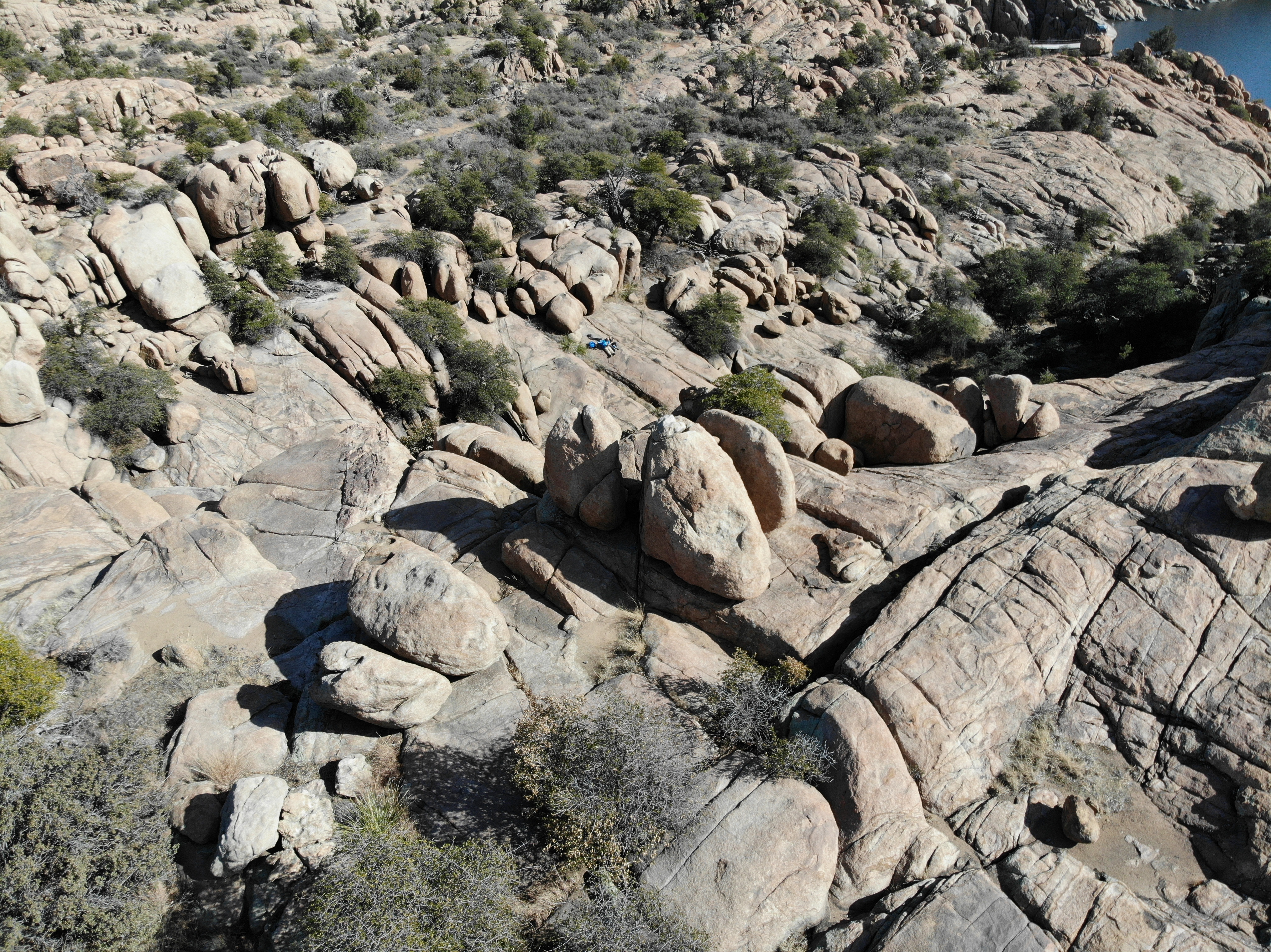
The fragility of geologic features, such as precariously balanced rocks (PBRs), can be measured by a simple parameter like α. For the case of a PBR is the smallest of the angles between the vertical from the center of mass and its rocking points. In a landscape, each object will have a fragility and so the ensemble will be a fragility distribution. The controls on the initial distribution and its long term evolution will be from the environment and its history (material properties, landscape evolution (lowering), weathering, shaking, etc.). The distribution can be disturbed by an earthquake (or other loading like windstorm, human impacts, etc.) which abruptly removes features with fragility below a threshold α.

Example of PBRs in Granite Dells, Arizona

I started to think an analogy with a fruit tree. I am not sure this is an original idea maybe I heard it somewhere. The progressive ripening of the fruit can be interrupted by a shake which will remove completely a subset of the most ripe fruit. For the case of the rocks, the ripening is a gradual decrease in fragility over time and then a fragility reset of a subset rather than removal after they are toppled in a shaking event. Ripening continues and the processes repeat over time. This simple model does not account for changing ripening rates or much variation in shaking effects other than threshold α. The basic idea then for seismic hazard is that the fragility distribution at a location reflects the history of the long term ripening and episodic shaking and reset. Therefore, if we can produce fragility distributions for landscapes that otherwise comparible (ripening and threshold α), we might be able to say which has seen more recent shaking and of what severity. This does not directly address the age control for the history and this remains a significant problem.

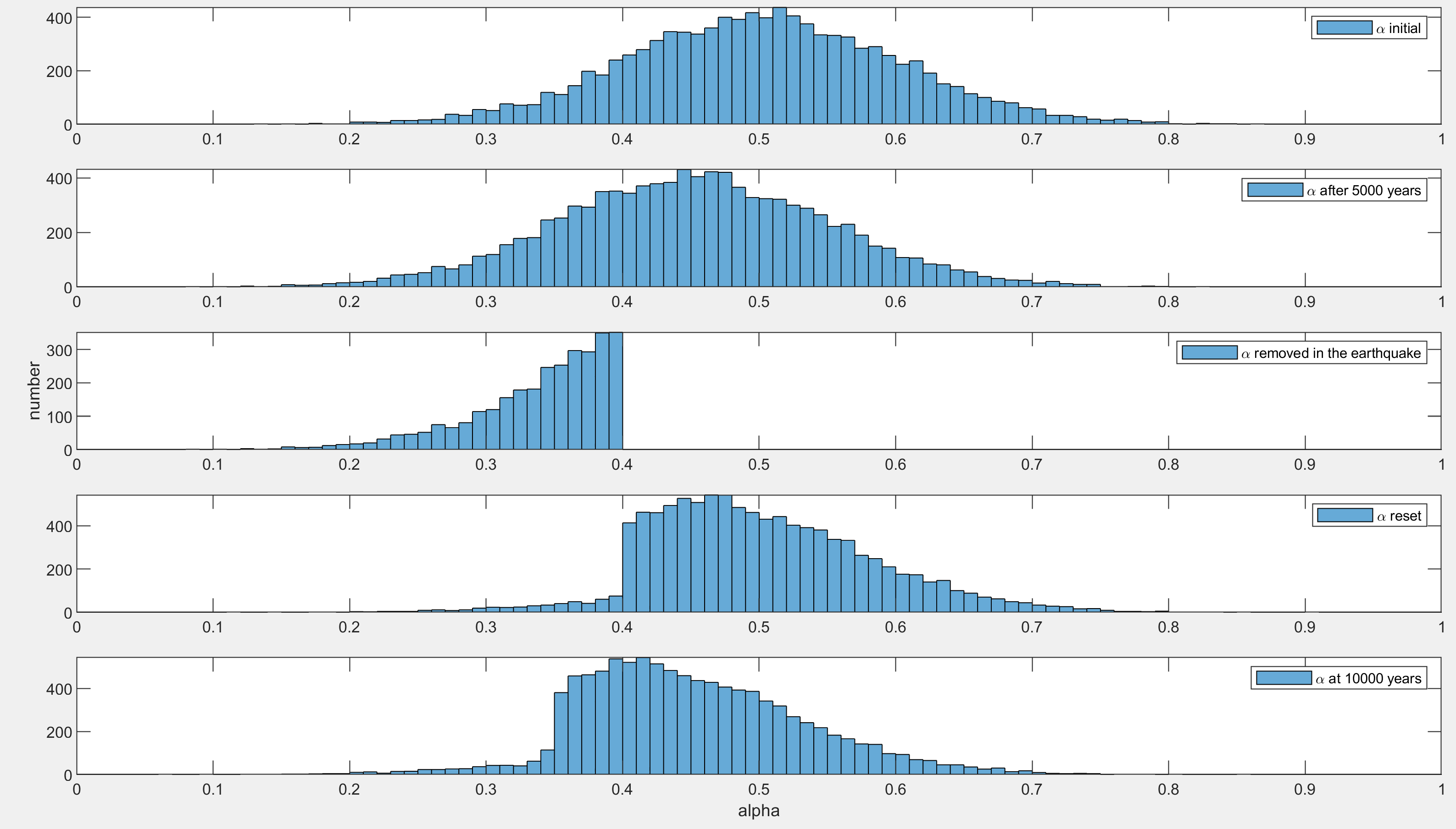
I wrote a simple code to explore this problem with the hope that it helps us explain and isolate the basic controls on fragility distributions. See the figure below which presents the fragility distributions through the experiment.The algorithm is simple:

• Set up: Specify number of objects, the initial α distribution (assume normal), the ripening rate distribution (also normal; this is the loss of fragility per year), the timing of the earthquake, the threshold α, and the max time
• Interseismic period 1: ripen α until the earthquake (begin and end are the upper two plots below)
• Earthquake: remove α < threshold α (third plot below) and reset those α drawing from the same initial distribution (fourth plot below)
• Interseismic period 2: ripen α until the end of the model time (final plot below)

Fragility distributions through the experiment. Upper plot is initial α. 2nd plot is α and the end of interseismic period 1. 3rd plot shows removed objects with α < threshold α. 4th plot is reset distribution of < threshold α Note that some α results below threshold α. Lowest plot shows continued ripening until the end of the model.

The additional two figures show the evolution of fragility with time of a subset of the objects and a spatial view of the randomly positioned features, their fragility at the time of the earthquake, and the circled objects that failed. The evolutionary diagram helps illustrate the interruption of the more fragile features by the event while the others do not notice. The map provides an idea of the search challenge that this scenario presents.

Evolution of fragility of a subset of the objects. The red star indicates the time of the earthquake and the threshold α.

Map view randomly positioned features, their fragility at the time of the earthquake, and the circled objects that failed.

Maybe more realistic with a more sparse set of features and a lower threshold α (0.3 as opposed to 0.4 above).

This is just a sketch of the problem, but it is a toy model in which we can explore the importance of the distribution widths, timing of earthquake, etc.

The MATLAB code is in this repository: https://github.com/jrarrowsmith/MATLAB-Geomorphology; make sure to get the script PBRevolution.m and functions ripenPBR.m and shakePBRs.

Eminent earthquake scientists: Clarence Allen and Robert Wallace oral histories

For some "light reading" over the winter break, I have enjoyed a read of oral histories of Clarence Allen (Caltech) and Robert Wallace (USGS).
EARTHQUAKES, MINERALS AND ME: WITH THE USGS, 1942-1995 by Robert E. Wallace; Oral History Interviews With Stanley Scott; USGS Open-File Report 96-260

Connections EERI Oal History Series: Clarence Allen with interviewer Stanley Scott
CLARENCE R. ALLEN (1925-2021) INTERVIEWED BY DAVID A. VALONE Caltech archives. This latter one has a bit more about Caltech and is slightly less polished than the first.

Maybe I at times too sentimental, but I found these personal and scientific histories throught provoking and inspiring, not only for their tellings of important steps in the history of earthquake science and service, but also for their modest, laconic, and matter of fact story telling. I am also fortunate to have substantial memories of interacting with both of them personally and also of the transition at the end of their careers and the beginning of mine (I entered graduate school at Stanford University in Fall 1989). I also appreciate the effort of EERI to accumulate those and other oral histories.

One thing that comes to mind is that it would be nice to include some histories from women who have contributed in these areas. I will work on that for a future blog post.

Bob Wallace was inspiring as an earthquake geologist. I followed some of his work quite closely as I shared an obsession with geomorphic indicators of faulting, although certainly with less of an impact...
Just a couple of examples from his papers:

1. 1949 - Wallace, R. E., Structure of a portion of the San Andreas rift in southern California: Bulletin of the Geological Society of America, v. 60, n. 4, p. 781-806.. This is cited as one of the earliest focused mapping efforts along the San Andreas Fault. He mapped substantial offset along the San Andreas Fault and also worried about the fault zone core and interactions of the drainage network with the fault zone. At one point, I colored the detailed map to appreciate it better.
2. 1968 - Wallace, R. E., Notes on stream channels offset by the San Andreas fault, southern Coast Ranges, California, in Dickinson, W. R., and Grantz, Arthur, eds., Proceedings of conference on geologic problems of San Andreas fault system: Stanford University Publications in Geological Science, v. 11, p. 6-21.. This was a landmark in my mind as he noted offsets along the San Andreas Fault in the Carrizo Plain as indicators of short and longer term indicators of recurrent fault slip. It was in a somewhat difficult to find publication. But, being around Stanford University (and having to move out of the Geology Corner after the Loma Prieta Earthquake), there were numerous copies to be found. Figures 6 and 7 of the histograms of numbers of channels with certain offset sizes was something we followed up on a fair bit.
3. 1990 - Wallace, R. E., (editor) The San Andreas Fault System, California: U. S. Geological Survey Prof. Paper 1515, 283 p.. This was his magnum opus. I was lucky once to meet him in his office at USGS Menlo Park and he asked if I had a copy yet. I did not even though I had stared at it. He reached into his filing cabinet and gave me his copy! I should have asked him to sign it or something but I certainly treasure that copy. It has now been rebuilt a few times...
4. 1992 - Wallace, R. E., Ground-squirrel mounds and patterned ground along the San Andreas fault in central California: U. S. Geological Survey, Open-file report n.91-149, p. 1-21.. This was a modest contribution, but I had a couple of conversations with him about it as we shared our enthusiasm for the Carrizo Plain. In his related GSA presentation, he even mentioned me as someone who might pick it up! Scared the crap out of me. We never really did a systematic effort on this but it remains a fascinating problem. I talk about it with people every time I get to the Carrizo Plain.

THere is a lot more to say and remember about Bob Wallace. My memories of him are also tied to Kerry Sieh who worked with Bob and honored him by naming the offset channel he explored in the 1968 paper "Wallace Creek". How many times have I read the Sieh and Jahns 1984 paper: Sieh, K. E., and Jahns, R. H. (1984). Holocene activity of the San Andreas fault at Wallace Creek, California. Geological Society of America Bulletin, 95, 883–896.. We even revisited this in our 2019 paper.

One of my San ANdreas Fault tour videos over the Carrizo Plain. Hillshades produced by me from the B4 project at OpenTopography.

I did not interact with Clarence Allen as much as I did with Bob Wallace, but I did have a few nice conversations with him. I think he was more serious in the conversations than I was. They main ones were when I was thinking about going to Caltech to work with Kerry Sieh. Clarence and I talked about science, but also about trout fishing. I regret never taking him up on an invite to fish in the San Bernardino Mountains. I think my father had fished some of the same places there around and below Lake Arrowhead or Big Bear Lake.
Two papers among many I would like to highlight from Clarence:

1. Allen, C. R. (1968). The tectonic environments of seismically active and inactive areas along the San Andreas fault system. Proceedings of Conference of Geologic Problems of San Andreas Fault System, 5(1496), 70–80.. This stands as an important first order characterization of the San Andreas Fault system and the recognition that the geology was an important control on the current behavior of the system. I have used Figure 1 here and there over the years when I kick of talks on the San Andreas Fault.
2. Geological Criteria for Evaluating Seismicity: Address as Retiring President of The Geological Society of America, Miami Beach, Florida, November 1974 CLARENCE R. ALLEN GSA Bulletin (1975) 86 (8): 1041–1057. This is a classic that helps to introduce the concepts of earthquake geology and the value of the geologic record in the study of recently active faults.

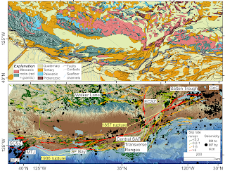
My recent attempt to follow Prof. Allen's ideas about the San Andreas Fault (some edits on the caption from Mike Oskin; we made this as a prototype for a SCEC request). The geology of the plate boundary shows the SAFS progressively dismembering the former subduction system (as indicated by the paired Mesozoic metamorphic--green and granitic--red rocks) (https://ngmdb.usgs.gov/gmna/; upper panel). This framework is a first order control on the behavior of the system (lower panel): active faults (USGS and CGS 2021) and M>4 seismicity (https://earthquake.usgs.gov/earthquakes/search/) overlain on the GMRT (Ryan, et al., 2009).

AI art: what does " Tectonic Geomorphic San Andreas Fault" look like?

I saw a link to https://app.wombo.art/ on twitter and people were posting what they got out of using their research or dissertation titles as a prompt. It is pretty amazing.

I gave it a try. My dissertation was entitled "Coupled Tectonic Deformation and Geomorphic Degradation along the San Andreas Fault System". I tried that as well as a shorter version "Tectonic Geomorphic San Andreas Fault" with a couple of different styles. I have to ponder the results. Some of the other examples work well when there is an object more recognizeable (such as a bird or T-cell), or somehow I need to give it a more interesting prompt. But the results are interesting. I like the trading card format.

Later on, I saw something about how the company could sell the "art" as NFTs but I guess I am not too worried about it.

Remembering Paul J. Umhoefer

I recently wrote this memorial for the Geological Society of America Structural Geology and Tectonics Division (which I am now beginning my stint as chairman or soon will). That is the reason for the first person plural.

We heard with great sadness and shock of the passing of our dear friend and colleague Professor Paul J. Umhoefer (Northern Arizona University) in late November 2021. Some of us saw him at the 2021 GSA meeting and to lose him so soon after weighs on us.

Paul Umhoefer was a great scientist, mentor and teacher, and servant to his professional community and department. He was well known for his research in tectonics, basin analysis, structural geology with carefully collected field data from the western US, Baja California, and Anatolia.

Much of his research was done in close collaboration with his many students at NAU. He was a strong mentor who guided many of those projects to publication and the students went on to success, especially in academia and the petroleum and geo-environmental industries. His professional colleagues appreciated his guidance and invitation to join interesting projects.

Paul was a tireless leader in the geoscience community. He helped to propel important community initiatives, including Margins/GeoPrisms. He not only contributed synthetic ideas but was an integrator and conciliator. He was an effective chair of his department helping guide it in a time of important growth. We are grateful for this leadership in the Geological Society of America Structural Geology and Tectonics Division where he was a long time active member, proponent of GSA fellows, and had recently completed the arc of leadership of the division.

Along with his tireless work ethic, Paul was enthusiastic and gregarious with a big smile and a joke for his friends and colleagues delivered in his deep creaky voice. He loved to talk about ideas: geoscience, politics, sports.

We counted on seeing him again soon. We are sorry to lose him and our thoughts are with his family and close friends.

Paul Umhoefer in one of his favorite places: the southern Baja California coast line with uplifted terraces and Tertiary sedimentary and volcanic rocks awaiting his attention (Arrowsmith photo, 2005)

--Ramon Arrowsmith (incoming Division Chair) on behalf of the Geological Society of America Structural Geology and Tectonics Division

Remembering Omar Abdullah

I heard in late August 2021 that Omar Abdullah was killed in the unrest that is occurring in Ethiopia. I did not learn of any details but he was an embasa--a lion--and no doubt he was there defending his family and lands. He was an amazing guy that I got to know over the years working in the Afar with the Ledi Geraru Project. Others knew him better. I appreciated him very much. He was from the Hadar woreda--administrative area--but we gave him a special title: "camp specialist" so we could keep him employed even when we were working in other areas with other Afars. Even the other Afars grew to appreciate him and his sense of humor.

Here are two pictures from 2002 (along with Mark Jakofsky). We can appreciate Omar's sense of fashion and poise.

Omar had a great sense of humor. There is a drainage called "Fat Ha'". It means big mouth in Afar. As Omar said, "like me!" He was also fascinated with our western scientist lives. He called himself "Black American." He was very friendly and happy to solve problems for the success of the project.

2006 pictures including Erin DiMaggio--she and I had lots of fun with Omar over the years!

We probably will not be back to Ethiopia and the Afar for a while sadly given the unrest. It will be very sad when we do and we really feel the loss of Omar (and probably others of our Afar friends). May he rest in peace. He always wanted me to bring him a small radio I think so he could listen to music while he waited for us to our work. I regret never quite getting around to that.

2009 and 2012 pictures including Erin DiMaggio and Matt Jungers.

NSF AC GEO Report on Portfolio Review of EAR Seismology and Geodesy Instrumentation Completed

In April 2021, we finished a fairly intensive project: AC GEO Report on Portfolio Review of EAR Seismology and Geodesy Instrumentation. I defer to that page as the official one, but I wanted to put a note here as well.

I was the chair of the committee, and the citation is

Arrowsmith, J R., Brodsky, E. E., Cooper, C. M., Elliott, J. L., Fee, D., Fischer, K.M., Hammond, W. C., La Femina, P., Lekic, V., Wang, H., and Worthington, L. L., Recommendations for Enabling Earth Science Through NSF’s Geophysical Facility – A Portfolio Review of EAR Seismology and Geodesy Instrumentation, Report to the US National Science Foundation, April 2021.

But, I want to really highlight the efforts of the entire committee! This was a really strong group that worked hard and respectfully together to come up with something we are quite proud of. It has some depth which I hope will give it shelf life.

Here are the rest of the Acknowledgements:
Thank you to UNAVCO President Rebecca Bendick and Director of Geodetic Infrastructure Glen Mattioli as well as IRIS President Robert Woodward and Portable Programs Manager Kent Anderson for their rapid and thorough responses to the committee queries. Christopher Crosby (UNAVCO) provided input on geodetic imaging. Jonathan Ajo-Franklin (Rice University), Kent Anderson (IRIS), Jnaneshwar Das (Arizona State University), Rob Evans (WHOI), W. Steven Holbrook (Virginia Tech), and Glen S. Mattioli (UNAVCO) kindly made themselves available for interviews with the committee. We are grateful to Lindsay M. Martin who supported the committee very ably as science assistant from the National Science Foundation. Finally, many thanks to Margaret Benoit (National Science Foundation Program Director) for her careful guidance.

Salt River terraces field geology exercise and updated guide

The Salt River in central Arizona has a spectactular set of fluvial terraces developed along it. I have lead a number of field trips along the Salt River for outreach and most importantly for our GLG451 Field Geology I course where we use a site along the Salt River for a mapping exercise. I have recently updated the materials associated with that exercise in anticipation of this Spring's class which will include a virtual component.

Tour from ASU to the Salt River site.

Drone overflight of the key sites for the exercise.

I built on some of the very nice writing and descriptions of Professor Pewe when I wrote up a field trip guide and ran a few field trips in the early 2000s. See this LINK. I updated that guide and it is available here: Landscape and geologic history along the Salt River near Tempe and Mesa, Arizona. I updated this document February 14, 2022.

Here is the assignment with many additional links and explanations: Virtual Field Geology assignment for Salt River Field Geology I 2021.
I made a long explanation of the GIS:

These were of great interest to Professor Troy L. Pewe of Arizona State University's Department of Geology. He moved to Arizona from Alaska and converted his research from permafrost to desert processes. I was lucky to learn from him when I first came to ASU in 1995. He took me under his wing and shared with me much of what he had learned. Most importantly, he helped me to learn the field trips and field sites he had developed and discovered. I am extremely grateful to him. I recognize Brian Gootee who was a great friend of the Pewe Family and who has preserved much of the Pewe legacy at the Arizona Geological Survey.

Pictures from those early field trips with Prof. Pewe.

Exploring diffusion for hillslope changes using a spreadsheet

I became obsessed with diffusion erosion modeling in my PhD work. It is a simple (certainly oversimplified) way to think about how hillslopes may change over time in the absence of mass wasting, debris flow, and fluvial processes. There is a lot to say about it, but I wanted to capture a few items I recently developed.

Here is an explanation and assignment on the topic in my Computers in Geology class: Lecture 8: Exploring diffusion using Excel.

One of the challenges that I have had in some applications is that the computational "space" was too small in the spreadsheet, given that it is fixed. Of course this is not a problem if one dynamically determines the number of time steps for example based on a stability criterion and you do it with a for or while loop in something like Matlab. So, when I was helping Emily Apel with her senior thesis recently, I built her a big spreadsheet (seemed easier given the limited time that she had.

Here is the original spreadsheet with only 27 space steps and 191 time steps. It is good for teaching and quick demos: LINK to Spreadsheet.

Above is the screen cap of the main interface page where the user just changes the bold cells and watches the calculations in real time.

Above is the screen cap of the Model Calculation Space tab which shows the compuational engine with its fixed elevation boundary conditions and explicit centered in space and forward in time finite differences.

Here is the big spreadsheet with 250 space steps and 1000 time steps: LINK.

And, here is a video that I built to explain the general activity for Emily Apel, but it may be useful for others. It explains the two spreadsheets that are linked above.

One of the cirtical concepts that is accessible in both of these spreadsheets is the opportunity explore not only initial step models, but also continuously displaced scenarios.

Here are a few other blog posts and recent publications which might be of interest as well:

• One dimensional morphological modeling of transport and production- limited fault scarps
• Updated review of fault scarp analysis
• Exploring the Topographic Evolution of Cinder Cones
• Some of my and my colleague's papers on these topics:
• Arrowsmith, J R. and Rhodes, D. D., Original forms and initial modifications of the Galway Lake Road scarp formed along the Emerson Fault during the 28 June 1992 Landers, California, earthquake, Bulletin of the Seismological Society of America, 84, 511-527, 1994.
• Arrowsmith, J R., Pollard, D. D., and Rhodes, D. D., Hillslope development in areas of active tectonics, Journal of Geophysical Research, 101, B3, 6,255-6,275, 1996. Correction: Journal of Geophysical Research, 104, B1, 805, 1999.
• Arrowsmith, J R., Rhodes, D. D., and Pollard, D. D., Morphologic dating of scarps formed by repeated slip events along the San Andreas Fault, Carrizo Plain, California, Journal of Geophysical Research, 103, B5, 10,141--10,160, 1998.
• Hilley, G. E., Arrowsmith, J R., Amoroso, L., The role of the interaction of normal faults and fractures on scarp morphology, Geophysical Research Letters, 28, p. 3,777-3,780, 2001.
• de Michieli Vitturi, M. and Arrowsmith, J R., Two dimensional nonlinear diffusive numerical simulation of geomorphic modifications to cinder cones, Earth Surface Processes and Landforms, doi:10.1002/esp.3423, 2013.
• Wei Zhanyu, Arrowsmith, J R., He, H., Evaluating fluvial terrace riser degradation using LiDAR-derived topography: An example from the northern Tian Shan, China, Journal of Asian Earth Sciences, Volume 105, Pages 430-442, 2015.
• Xu, J., Arrowsmith, J R, Chen, J., Schoenbohm, L. M., Li, T., Yuan, Z., Evaluating young fluvial terrace riser degradation using a nonlinear transport model: With application to the Kongur Normal Fault in the Pamir, northwest China, Earth Surface Processes and Landforms, DOI: 10.1002/esp.5022, 2020.

Simple computations of scalar seismic moment and moment magnitude

In my classes and for research, sometimes it is useful to calculate the scalar seismic moment (M₀; basically a geometric measure of the total static energy release at a 0th order). It is a function of the area of a fault that slipped times the average slip times the shear modulus of the volume. The latter is usually assumed to be 30GPa. The main challenge (after determining the parameters) is to get the units all to be the same (dimensions of Newtons and meters):

M₀= mu*Length*Width*U_bar.

And, once we have that scalar moment in Nm, then we usually want to convert it to moment magnitude (M_w):

M_w = 2/3 log10(M₀) – 6.

Here is a simple spreadsheet to do this calculation: LINK
Here is a simple and older lecture I have used in introductory level geoscience courses: LINK

New fast workstation and sUAS capability for School of Earth and Space Exploration course development

Overview

Our geoscience courses have benefited from plenty of course development, especially lately as we have moved online and virtual. I recently was able to invest SESE course fees to build out our capabilities for high resolution mapping and 3D work. Javier Colunga built a nice and fast Windows workstation, and we also purchased a Mavic Pro 2 sUAS system. The descriptions are below for reference.

Workstation description

We have been building these "gaming" style fast desktops for a while and this latest incarnation is powerful for graphics intensive and 3D work, especially structure from motion photogrammetry (e.g., Johnson, et al., 2014 and GSA short course).
Here is a short description of the hardware (cost approx. $5k):

• CPU: Ryzen Threadripper 3970X 32-core/64-thread (with a premium cpu cooling solution)
• Main Memory: 128GB DDR4 3600
• Graphics Card: GeForce RTX 2080 Super
• Storage: Samsung 1TB M.2 NVME OS drive, additional 4TB hard drive
• Operating system: windows 10 Enterprise
• Input: Logitech wireless keyboard and mouse
• Monitor: HP 27 inch 1440P

Here is the main software installed:

• Google Earth Pro
• Matlab R2020a
• Camtasia 2020
• Cloudcompare
• Agisoft Metashape
• ArcGIS 10.7
• QGIS

Here is more description, how to connect remotely, and a sign up sheet. LINK

sUAS description

For SESE, we have purchased a DJI Mavic 2 Pro (actually the FlyMore combo so it has a nice case and 3 batteries). This is a nice mapping and aerial documentation system.

Devin Keating has been helping to get the system into production mode. He has built a nice documentation of the system and its use. He also registered it with the FAA so we have a tail number. See this LINK. To operate it, one should have the part 107 Remote Pilot certification. And, there are ASU oversight requirements as well.

Recent course related work using this type of system (and computed on the nice workstation described above):

Warford Ranch volcano (Arizona) sUAS mapping

Virtual field geology exercises for GLG451 Field Geology I Spring 2020

Material for virtual exercises for GLG452 Field Geology II at Camp Tontozona AZ

Warford Ranch volcano (Arizona) sUAS mapping

Introduction

We recently visited the Warford Ranch Volcano which is a low shield volcano that is part of the Sentinel-Arlington volcanic field of southwestern Arizona. It is about 3 million years old. It was a favorite field trip destination of Prof. Ronald Greeley. Shelby Cave worked on the Sentinel-Arlington field for her Ph.D. dissertation under the supervision of Prof. Greeley and after his passing she worked with Prof. Amanda Clarke.

Google maps location for Warford Ranch (NW of Gila Bend, AZ).

Professor Clarke is teaching the Advanced Field Geology course and she took the group to Warford Ranch volcano to examine its volcanology. I did some UAS-mapping to help with the documentation. This blog entry presents some of the products of the overflights with our Mavic Air and Phantom 4 Pro.

Oblique overviews

I flew the Mavic Air high to get some views over the volcano to assess its general form and the relation to adjacent landforms and geology.

View to the north. The cars are lower left are in our parking spot. LINK to jpg

View to the south-southwest. LINK to jpg

View to the south-southeast. LINK to jpg

Fissure zone on SW side of higher topography. People for scale. Not sure the purpose of the excavation. LINK to jpg

Masked and socially distanced field work. LINK to jpg

Video overflight.

sUAS mapping

Along with the free flying overviews, I flew in mapping mode (using the PX4D mapper app) over most of the volcano taking 1778 images in mapping mode. I processed those in Agisoft Metashape to produce a colored point cloud, digital elevation model, and orthophoto. The latter two can be the basis of more mapping in ArcMap.

Tour of the data and its processing in Agisoft Metashape and ArcMap.

Map downloads

Hillshade overview. 600 dpi pdf download: LINK.

Ortho image overview. 600 dpi pdf download: LINK.

Hillshade of peak area. 600 dpi pdf download: LINK.

Ortho image of peak area. 600 dpi pdf download: LINK.

Map data downloads

• 0.1 m/pix DEM and hillshade downloads (tif): LINK
• 0.1 m/pix orthoimage download (tif): LINK

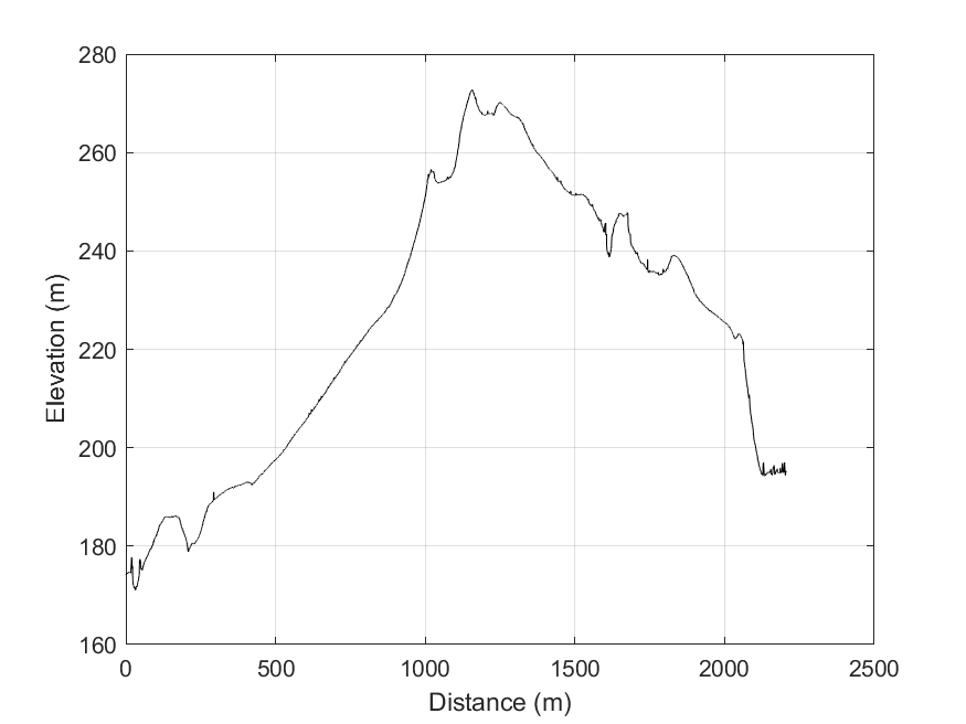
Topographic profile

The video presented above discusses the topographic profile cut from the DEM in ArcMap towards the end. This would be the basis for the geologic cross section, preferably without vertical exaggeration.

Topographic profile location. Bent along the path of our Saturday November 22, 2020 tour. LINK to png.

Topographic data text file: LINK and MATLAB script to plot it: LINK

No vertical exaggeration. Link to png.

Vertical exaggeration. LINK to png

2021 ADDENDUM:
For the October 2021 field work, we are trying to use STRABOSPOT for the digital mapping. I prepared a few items to help:

• Simple tutorial. The students need to do all but the very last step (uploading after the field) BEFORE we go to the field: PDF
• Video tutorial. I recorded all of this on the browser and the tablet with narration.