Monday, December 16, 2019

Call for research papers: Unveiling Active Faults: Multiscale Perspectives and Alternative Approaches Addressing the Seismic Hazard Challenge

Along with Federica Ferrarini, Nathan Toké, and Michele M. C. Carafa, we are looking forward to submissions to this special "issue" from the Frontiers journal: Unveiling Active Faults: Multiscale Perspectives and Alternative Approaches Addressing the Seismic Hazard Challenge.

Federica made a nice flyer to share: LINK


Central Apennine settled landscape with active normal fault (photograph by Federica Ferrarini).

Despite decades of progress toward mitigating seismic hazard, characterizing the seismic potential of an area remains a complex process. Particularly challenging are seismically active regions characterized by low slip rate faults which can give rise to weak geomorphic expressions when combined with high erosion or sedimentation rates. Similar compounding issues may also manifest in densely populated areas where anthropogenic modifications, or vegetation cover further challenge assessment of fault activity or where structural complications may contribute to multiple interpretations. Noticeable advances in remote sensing technology geodetic measurements and dating Late Quaternary landforms and sediments have moved our understanding forward.

This Frontiers Research Topic welcomes contributions that present examples and approaches which strive to improve our understanding of active faulting processes over diverse geological settings and at broad spatial scales of investigation. We encourage the submission of research papers from a wide range of geoscience disciplines (field geology, structural geology, tectonic geomorphology, paleoseismology, seismology, remote sensing, numerical modeling) and from the scale of a field site to regional scale analyses. We welcome contributions with the main goal to bridge the gap between our observations, fundamental understanding of faulting processes, and effective seismic hazard assessment.

Please think about a contribution! Submit an abstract by January 29, 2020 (not required). The manuscripts are due May 29, 2020.

Saturday, October 5, 2019

(Finally) Getting going with python (and a bit of history)

I certainly recognize the power of scientific programming. Programming spreadsheets is obvious and there is nothing to be ashamed of there (see weeks 2-6 in my Computers in Earth and Space Exploration course). I started off in grad school with Mathemematica and appreciated the notebook style of computations and integrated graphics and text. I also taught myself enough fortran to get the main calculations for my dissertation completed.


Modeling profile development with simple diffusion (Arrowsmith, et al., 1998) using fortran code and Mathematica for the basic graphics.

I took some programming courses (Pascal) back in grad school. I was not very good at it. Once the professor even said "that is the stupidest way I have ever seen for doing that" in office hours. I was not too offended; I barely understood what I was doing. Nevertheless, I got the big picture and have stumbled along ever since.

Professor George Hilley taught me many things. One thing he was able to do after a fair amount of cajoling was to get me to start in MATLAB. The more data-oriented and matrix handling of MATLAB ended being something I could use effectively. We also worked with Don Ragan a lot on MATLAB and Latex. While I am no expert, I have taught the basics to students over the years see weeks 6-9 in my Computers in Earth and Space Exploration course). I cannot say that I have had any really great programming projects, but the various analysis and plotting needs have been satisfied. For what it is worth, I even set up a GitHub page to hold a few things. Dr. Olaf Zielke is a serious MATLAB programmer and wrote some impressive tools with GUIS for his PhD and related work. TopoToolbox is another set of MATLAB-based tools which I had the opportunity to learn and appreciate their transformative power for a lot of geomorphic analyses.

I have been watching the progressive adoption of Python and related tools in my little scientific bubble over the last 5 or so years. I have not had the time to do much as far as learning until recently, however. While my MATLAB expertise won't go away, I have appreciated the fact that it is hard to share and teach with students and colleagues who don't have access to the rather expensive licenses for MATLAB. On the other hand, Python and related tools are open and apparently so adaptable and customizeable.

Recently, I finally had an excuse and the time to get my feet wet with Python. Chris Crosby and I (OpenTopography) helped out with a short course From point clouds and full-waveform data to DEM analysis (Sep-30 to Oct-4 2019) led by Professor Bodo Bookhagen and his team.


Specific catchment area computed with the tools from Rheiwalt, et al., 2019. The basic processing was in Python with some c code and then visualized using Displaz.

Here is some basic full waveform lidar processing from Bookhagen and Rheinwalt again basic procesing in Python and then visualized using Displaz.

I still don't understand all that I am doing, but I got the basic set up and can sort of understand packages and environments. Javier Colunga helped me by getting Ananconda installed. Spyder is the development environment I had been looking for. There is so much that is possible; it is hard to even know where to start.

For my first project, I thought it would be nice to play around with a lidar point cloud (using the Dragon's Back of course): grid it using pdal and then make a hillshade using gdal. Download the data from OpenTopography.

The steps are:

  1. Launch an Ananconda terminal.
  2. Add these conda channels for package install:
    conda config --prepend channels conda-forge/label/dev
    conda config --prepend channels conda-forge
  3. Then define an environment and add the packages using conda: conda create -y -n PC_py3 python=3.6 pip scipy pandas numpy matplotlib scikit-image gdal pdal xarray packaging ipython multiprocess h5py lastools pykdtree spyder gmt=5* (this comes from the workshop).

My first problem was that I could not run pdal from inside a python script. There is something I don't understand there (even though it is installed, etc.). I see that it is possible to call python from inside the pdal json files... But, I can run it from the command line:
> pdal pipeline db.json
where the db.json has the parameters for the simple neighborhood gridding run:


{
        "pipeline":[
        "smallpiece.laz",
        {
                "resolution": 1,
                "radius": 0.707,
                "gdaldriver": "GTiff",
                "gdalopts": "COMPRESS=DEFLATE, ZLEVEL=7, GDAL_NUM_THREADS=ALL CPUS",
                "data_type": "float",
                "output_type": "idw",
                "filename":"small_idw_1m.tif"
        }
        ]
}
I was able to make a little dem (the tif file). But then, I ran the gdal from the command line only:
>gdaldem hillshade small_idw_1m.tif small_idw_1m_shd.tif

Finally, I could run a little python script to draw the hillshaded geotiff (this I could run from Spyder):


#!/usr/bin/env python
import gdal
import matplotlib.pyplot as plt

ds = gdal.Open('small_idw_1m_shd.tif').ReadAsArray()

plt.close('all')

plt.imshow(ds, cmap='gray')

f.savefig('smallDB.png', dpi=300)
plt.close('all')


Small piece of the Dragon's Back lidar data (B4 project) gridded with pdal, hillshaded with gdal, and drawn with matplotlib

So, I guess that is a bit of a success, there is a lot more to do and learn!

I keep finding references to help learn:

Monday, September 23, 2019

Many thanks to Petroleum Experts Limited

Petroleum Experts Limited has provided the School of Earth and Space Exploration with licensed software for 2D and 3D kinematic modelling, geomechanical, fracture, and fault response modeling and fault and stress analyses. These licenses are valued at $2.18M and will enable our faculty and students to build and analyze complex 3D fault models to develop understanding of tectonic processes and to anticipate earthquake hazards.

Here is a LINK to our SESE newsletter acknowledging the donation as well

We are really grateful for this donation. The MOVE suite of software is a powerful environment for 3D interpretation. My students and colleagues are using it to build 3D fault models. We hope to begin to work on sedimentary architecture in extensional environments in the coming year. In addition, with continued support of the licensed software, we will develop course material for it for our geology majors.


Example image from Petroleum Experts/MOVE.

Thursday, July 4, 2019

Remembering Donal M. Ragan

Professor Emeritus of Geology Donal M. Ragan passed away in February 2019. Unfortunately, I had lost some contact with him in the last years. However, I was first hired on in 1995 at ASU to take Don's position (from which he had retired) and teach Structural Geology. He was still active, working on his book and so he came by often to talk with me and my students (especially George Hilley). Don and his wife Janne were also kind to have me over for dinner occasionally. They were very generous. This memory of Don is incomplete, but I wanted to capture a few thoughts and recollections.

This is the only picture I could find of Don. He is there on the left (along with Lee Amoroso, Jeri J. Young, and George Hilley) during a field trip to the Carrizo Plain in the late 1990s.

I don't have all of Don's biography. I recall he was born in southern California and maybe went to Occidental College. He was in the Army and talked about the discipline and repetitiveness of learning how to dissassemble and assemble a machine gun. He went to the University of Washington where he worked on deformation in the Twin Sisters Dunite. He was at Imperial College where he worked with John Ramsay. He moved to the University of Alaska (UAF) and published on deformation associated with glacial ice (e.g., Ragan, 1969). He moved to Arizona State University in 1965 at the behest of Prof. T. L. Péwé who had been hired to be chairman and who knew Don from UAF.

We worked a fair bit with Don on MATLAB implementations of his exercises and ideas. A couple are here. And, he was an avid LaTEX user having had problems in the 3rd Edition of the book when he did not have good control over the copy editing and production. He taught us about dashes and quotes.

In 2000, Don taught a series of lectures on Structural Geology. I helped a bit mostly as coordinator and provider of moral support. These reflected the development for the book and all I really have are the handouts and figures for transparencies and a few notes:

Don was outspoken about quantitative approaches in structural geology: "Despite all this effort one can still find in professional articles statements that violate basic laws of physics and in some current textbooks there are important omissions, misstatements, misinterpretations and errors when dealing with structure making processes." (from his review of The Life of Frank Coles Phillips).

I worked with him for a while on the 4th edition of the textbook, but did not contribute enough in time to stay a coauthor. Nevertheless, I learned so much from Don and did what I could to apply those lessons in the GLG310 Structural Geology and the GLG510 Advanced Structural Geology courses. We talked often about how to teach structural geology and how to bring more quantification and precision to it. We followed the developments of the structural geology textbook (FSG) of Professor David Pollard at Stanford. Don and I wrote a short review of an early version of a manuscript on kinematics and mechanics here. Don wrote a blurb for the book: "This is the best book on structural geology in a long time. It is both rooted in classical mechanics and visionary. In their characteristic fashion, Pollard and Fletcher lay out the physical concepts and tools needed to understand the structure-making processes and give many examples of their use. If you have any interest at all in the subject read this book, but be prepared to work. You’ll be glad you did."

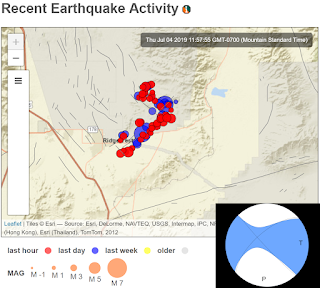
M 7.1 - 17km NNE of Ridgecrest, CA (was Accumulating links for: M 6.4 - 12km SW of Searles Valley, CA)

I have prepared a summary presentation on the earthquake sequence. The July 17 versions here here: PDF and PPT. They are comprised of material harvested from publicly accessible sites, so I am hoping it is ok to redistribute in this form; I have provided attribution. Let me know if something needs to be udpated.


And then the the 4th of July event was a foreshock. As I mentioned below, there was a 9% probability from the USGS that the July 4th event would be followed by something larger, and it actually was. I hope that people are ok; will take until the morning to have a better sense of damage and injuries.

I am regularly updating this page, so occasionally refresh.

Tonight's event is clearly part of the same sequence, although this was along the NW-trending section (and was right-lateral). This is an impressive conjugate pattern (right lateral along the NW orientation and left lateral along the NE orientation). Both orientations and senses of motion are consistent with the overall shear zone deformation in the area. It looks to have ruptured across the Highway 178. There are also lots of mass movements in the area (lots of dust kicked up in videos, and also rock falls onto the roads, etc.).

This event was an M6.9 refined from the M7.1 initial estimate. This is a half magnitude unit larger so it was ~10x more energy, hence the broader felt extent (more people in Phoenix and Las Vegas noted it; e.g., my colleagues and my sister...). If you felt (or not) good to fill out a report. This one will certainly be followed by many aftershocks, and there is again a small chance that a larger one could follow. (Omori’s law: ~logarithmic decay in time for event rate (ratio of big to small aftershocks stays the same.) But you can also think of these events close in time and space as epidemics (epidemic type aftershock sequence, most that follow are smaller, but sometimes a bigger one can follow as we have seen). An event of the July 4 size could be an aftershock now...

Locations from http://www.scsn.org/ and the focal mechanism from USGS. Compare this with the similar one below.

ASU recording: http://earthquake.asu.edu/EQplots/ci38457511.pdf; thanks to John West and Ed Garnero

~~~~~~~~~~~~~~~~~~~~~~~~

A 4th of July earthquake with an impressive conjugate aftershock pattern in the Eastern California Shear Zone.

Locations from http://www.scsn.org/ and the focal mechanism from USGS.

Deferring to USGS/CGS colleagues for the real interpretation, but this looks to be consistent with maybe a primary rupture on one of the trends and then aftershocks climbing up the other. Given the magnitude and length scaling, for the moment, I am going to guess the rupture was on the NE trend and would be left lateral with a few 10s cm cracking (based on image below could be Little Lake Fault zone?). This is also consistent with the conjugate fault pattern mapped in the region (see NW and NE-trending faults on map below).

Update about 2 pm: indeed, decimeter-scale rupture, left lateral, crossing Highway 178. See this tweet. The location is 35.644167, -117.535833--close to where the aftershock trace.

It has a vigorous aftershock sequence which is consistent with expectations. The USGS is employing Operational Earthquake Forecasting to provide probabilistic statements about expected aftershocks in the region.

Locations and active faults from USGS. Fractured Hwy 178 from @neotectonic

It was widely felt in California: USGS DYFI. This is a good reminder about earthquake safety.

Useful links:

Sunday, March 17, 2019

From crashing kites and Frankenmodels to efficient large-scale UAV acquisitions and beautiful shared 3D models (2018 GSA talk)

I was invited to give a presentation in a session at the Fall 2018 Geological Society of America session T60. Revolutions in Remote Sensing: Applications of UAVs to Field Mapping and Surface Analytics (organized by Dylan Blumentritt--Winona State University and Toby Dogwiler--Missouri State University). I decided to make a my presentation a bit of a reflection of how my own obsession with low altitude imaging had evolved and how far we had come. After all, I started in college working in the Fairchild Aerial Photography Collection when it was at Whittier College. So, I came up with a talk with the hopefully entertaining title of FROM CRASHING KITES AND FRANKENMODELS TO EFFICIENT LARGE-SCALE UAV ACQUISITIONS AND BEAUTIFUL SHARED 3D MODELS. I am putting links to the talks on line in case they might be useful: PPT and PDF.

The presentation shows a couple of maybe interesting things:

  1. It shows a pretty 3D point cloud (video above) from our Photogrammetric model of the Tecolote Volcano, Sonora, Mexico hosted at https://opentopography.org/.
  2. It spends some time talking about and making the case for the OpenTopography Community Dataspace.
  3. As part of the OpenTopography Community Dataspace discussion, I (with slides and ideas from Chris Crosby) talked about standardizing metadata for these long tail data. See for example the different styles of metadata documents ("Survey Report"): for example Almaty range front fault, Koram site or Clear Creek, Idaho post-fire debris flow erosion--note the ones I uploaded are not great examples :).
  4. Of course, one of the really nice things that the OpenTopography Community Dataspace publishing of one's data allows is to mint a DOI. That DOI allows then for a data citation. I have added a new part of my CV that has a section on data publication. Here is an example citation style:
    Arrowsmith, J R., DiMaggio, E. N., Garello, G. I., Villmoare, B. and LediGeraru Research Project (2018): Photogrammetric model of a portion of the LeeAdoyta Basin, Afar, Ethiopia (point cloud [122M points], orthophoto [2cm/pix], and DEM [25 cm/pix]). Distributed by OpenTopography. AccessedOctober 23, 2018. https://doi.org/10.5069/G95X271W.

The conclusions are useful to highlight as well:

  • We are part of a revolution in 3 and 4 D data collection and analysis
  • Additional needs for the community include
    • Optimized data acquisition strategies
    • Low cost and high performance computation of point clouds and models
    • Efficient and accurate georeferencing
    • High quality differencing for change detection
    • Bring the tools and data into the (outdoor) classroom; need more curriculum (c.f. GETSI - GEodesy Tools for Societal Issues (UNAVCO) at https://serc.carleton.edu/getsi/)
  • OpenTopography Community Dataspace
    • Great opportunity to expand the impact of emerging topography through improved access
    • Services and existing community of users
    • Community engagement & best practices
    • Please join us and start sharing your models and ideas for how to improve

Monday, March 11, 2019

Anniversary of Great Tohoku Japan earthquake and tsunami (20110311)

Today is the anniversary of the catastrophic great Tohoku Japan earthquake and tsunami of March 11, 2011. While I am not an expert of subduction systems nor tsunamigenesis, I was of course interested in the event and prepared some lectures about it. While there are many better and newer illustrations, I wanted to share the materials.

The first presentation was at the Arizona Science Center in 2011. Here is the folder of the materials.

I prepared a lot of content for a series of lectures at IT Bandung in Java that I presented in 2013 with the help of my former student Dr. Gayatri Marliyani. There is much high quality material at IRIS (some of which I have included). The main materials are in these three folders:

Friday, March 8, 2019

Idea for an earthquake intensity exercise based on 1857 Ft. Tejon earthquake data

I was cleaning some files yesterday and I found an old exercise I had deployed when I was first teaching Introductory Geology. It was intended to help students understand earthquake intensity (vs.) magnitude. I took the felt intensities as reported by D. C. Agnew and K. Sieh (1978), A documentary study of the felt effects of the great California earthquake of 1857, Bull. Seismol. Soc. Amer., vol. 68, pp 1717-1729 and compiled some of the more easily interpreted ones into a table and then provided a simple map of California for the students to map the intensities. Here is a link to the compiled data from Agnew and Sieh. THe work of Kerry Sieh on the 1857 earthquake is seminal. I think it was an ok exercise, but there are probably more interesting and more recent datasets. For example, I like the twitter-based work that is coming from the USGS colleagues. It should be possible to take some sample tweets and do an intensity mapping.

The 1857 earthquake and its foreshocks and aftershocks are fascinating an a sobering reminder of what will happen one day in California.

This figure from Toké and Arrowsmith, 2006 shows the 1857 foreshocks and the mainshock distribution (the latter is what the exercise mentioned in the last paragraph is supposed to look like) and compares it with the historic Parkfield earthquakes.

Monday, February 25, 2019

Updated review of fault scarp analysis

I am organizing for a presentation to my research group on fault scarp analysis. This is an ongoing obsession of mine. I have blogged about this topic here with some review. That is still a pretty good summary of things. I also have a couple of relevant Landers Earthquake posts here and here. And, we applied many of the relevant tools to analysis of cinder cone forms.

The 2017 post mentioned above is still a pretty good summary of things. However, the MATLAB-based guis for Penck1D and Scarpdater are not running well now on newer versions of MATLAB; they need an overhaul. We were really into guis back then but they require so much code relative to the actual modeling. Might be cool to rewrite in Jupyter notebooks, maybe see how much in landlab could be used.

I have prepared a new review powerpoint (PPT and PDF) with this outline:

  • Introduction and review
  • Diffusion-equation analysis of scarplike landforms
  • Observations
    • Direct dating of fault scarps
    • Fault scarp erosion monitoring
  • Modeling
    • Distributed deformation
    • Transport vs. Production limited
  • Extending processes 2D and nonlinear diffusion
  • Prospects and cautions
Of course it is incomplete and emphasizes the work of my students and colleagues. I note for example, this nice review from Wei, et al., Journal of Asian Earth Sciences, 2015:

Additional resources for my lecture include:

Some other useful web links include: