Structure from Motion using video from my phone camera

Introduction. In my last post, I showed how I had extracted frames from satellite-derived video to build a 3D model of a mine from space. In this post, I show a similar workflow for phone camera: take a video of an object (some times a lot easier than numerous frames although lower quality) and make a 3D model using Agisoft Photoscan.

Video to images. (this part is repeated from the last post). The main generic challenge for SfM from video is to extract the video frames and prepare them for the SfM. The SfM part is no different from what my group has been doing for a while with Agisoft Photoscan. I used MATLAB to do the video processing. The script is here: readplanetvid.m. The main code bits include:
PlanetObj = VideoReader(videoname); %make a video object from an MP4 file
vidWidth = PlanetObj.Width; %get the width
vidHeight = PlanetObj.Height; %and height

mov = struct('cdata',zeros(vidHeight,vidWidth,3,'uint8'),...
'colormap',[]); %set up a MATLAB structure to contain the video

k = 1;
while hasFrame(PlanetObj)
mov(k).cdata = readFrame(PlanetObj); %pull out the frames one at a time from the MP4 object and put them in the mov
k = k+1;
end

step = floor(k/number_of_frames) %determine how many frames to skip each time to get the desired number
for i = 1:step:(k-1)
framepart = sprintf('_frame_%06d.png', i);
filename = strcat(foldername,'/',projectname,framepart);
imwrite(mov(i).cdata, filename) %easy to write the frame out as a png file
end


Video of a rock sample in my backyard. I took a short video of a piece of obsidian on a table with my Samsung J3. The nice thing about it was that I could gather a large number of views around the sample with relative ease. From that video, I extracted 150 frames, for example see below

I ran the files through the Agisoft Photoscan sequence of alignment (high), build dense cloud (medium), build mesh (medium), and build texture (medium). Here are a few screen captures of the result:

This one shows a somewhat complex background, but nicely indicates the path of the camera too.

And here it is with a trim to only show the sample on the table:

Structure from Motion using video frames; MATLAB for frame grabs and an example from satellite video

Introduction. Occasionally we and also we have gotten a question as to whether it is possible to use video frames as input for Structure from Motion models. This has certainly been done before with good success. For example, Yuichi Hayakawa did it starting with news video for a landslide triggered by the Kumamoto, Japan Earthquake in April 2016. Roman DiBiase showed me how he had done it video from helicopter and even performed topographic differencing with lidar for the Big Sur Landslide (e.g., NPR site and USGS site).

So, in a fit of procrastination, I decided to play around with the process myself. I was motivated originally by an idea from Andrea Donnellan and others at JPL to do topography from satellite video. They wrote a report entitled Gazing at the Solar System: Capturing the Evolution of Dunes, Faults, Volcanoes, and Ice from Space and I worked with Andrea and her team some on the problem.

Video to images. The main generic challenge for SfM from video is to extract the video frames and prepare them for the SfM. The SfM part is no different from what my group has been doing for a while with Agisoft Photoscan. I used MATLAB to do the video processing. The script is here: readplanetvid.m. The main code bits include:
PlanetObj = VideoReader(videoname); %make a video object from an MP4 file
vidWidth = PlanetObj.Width; %get the width
vidHeight = PlanetObj.Height; %and height

mov = struct('cdata',zeros(vidHeight,vidWidth,3,'uint8'),...
'colormap',[]); %set up a MATLAB structure to contain the video

k = 1;
while hasFrame(PlanetObj)
mov(k).cdata = readFrame(PlanetObj); %pull out the frames one at a time from the MP4 object and put them in the mov
k = k+1;
end

step = floor(k/number_of_frames) %determine how many frames to skip each time to get the desired number
for i = 1:step:(k-1)
framepart = sprintf('_frame_%06d.png', i);
filename = strcat(foldername,'/',projectname,framepart);
imwrite(mov(i).cdata, filename) %easy to write the frame out as a png file
end


Satellite video from Terra Bella. I have been watching the hi resolution satellite activity with great interest. Skybox had a few relatively high res (approx 1 m ground resolution) visible and near IR satellites with video capability. They were bought by Terra Bella (google) and then now are owned by Planet (who were just visiting us on the ASU campus last week and with whom we are building some collaborations). Some of the Terra Bella imagery is available on youtube. I grabbed one video of the Usak Mine in Turkey (used real player to convert youtube to mp4):

You can really see the parallax as the satellite moves over (not to mention the activity of the vehicles).

I ran my script on the mp4 and extracted 100 png frames. Here is an example:

I ran the files through the Agisoft Photoscan sequence of alignment (high), build dense cloud (medium), build mesh (medium), and build texture (medium). Here are a few screen captures of the result:

You can see the model and the camera positions. They are in the roughly correct arc, and relatively far away, but they should be much farther (orbit is approx 450 km).

Nice looking textured mesh. It is distorted, but not too bad, all things considered!

And, here is the point cloud in Cloud Compare.

What did we learn? We learned that the SfM from video is doable (see a future post from my backyard and phone video). Here is the Photoscan report on the Usak project. The geometry that is computed from the satellite video is not bad. Agisoft Photoscan does a pretty good job. We cannot get under the hood very easily to see more about the processing. I think that someone who knows more about computer vision than me would be able to comment as to the performance. I think that the main issue is probably the relatively low angular variation for the model.

Planet Team (2017). Planet Application Program Interface: In Space for Life on Earth. San Francisco, CA. https://api.planet.com.

M 8.0 - west central Mexico coast offshore Chiapas

A great earthquake has occurred off of the west coast of Mexico offshore of Chiapas. It is tsunamigenic. It looked to be along the subduction interface, but the focal mechanism and depth suggest normal faulting in the slab below. See seismicity map for more commentary about normal faults and this cross section.
I am accumulating some links here. Check back for more.

From USGS

Recording at ASU

IRIS Teachable Moment materials for this earthquake

Links:

• USGS main page on the event
• USGS finite fault model
• IRIS back projection model
• US tsunami warning system--apparently no imminent tsunami danger for western US
• European-Mediterranean Seismological Centre page on the event
• GeoScope page on the event--has nice source time function
• Bravo, et al., 2004 paper on Tehuantepec portion of Mexican subduction zone.
• Nice map and tweet from Steven Hicks
• Nice interpretations from EarthJay
• Mountain Beltway blog explainer
• Temblor blog explainer
• Webcam de Mexico shows 2 minutes early warning
• KQED news report
• Cool comparison of earthquake and hurricane seismograms

Some new San Andreas Fault tour videos of 1 m bare earth hillshades

I have been preparing a lecture and I built some new simple videos flying along the San Andreas Fault. The videos are made by me flying along in Google Earth with 1 m hillshades produced from lidar topography data collected along the San Andreas Fault. The videos are on youtube in this play list: https://www.youtube.com/playlist?list=PLFfZSFyNZ_jZm86F1TsnYfuuYNef_Uh21. I also put the MP4s in this folder--they are numbered 1-8 from NW-SE.

The flights follow generally along the San Andreas Fault from Point Arena to the southern Carrizo Plain (Dragon's Back and Northern Elkhorn Hills):

The data were processed at www.opentopography.org and come from 3 really cool datasets:

• EarthScope Northern California Lidar Project. Data collected by National Center for Airborne Laser Mapping.
• B4 project: southern San Andreas Fault laser scan. Data collected by National Center for Airborne Laser Mapping in collaboration with USGS, UNAVCO, and Ohio State University.
• Dragons Back Ridge: San Andreas Fault, California acquisition. Data collected by National Center for Airborne Laser Mapping in collaboration with George Hilley.

One dimensional morphological modeling of transport and production- limited fault scarps

Over the years, I have maintained a steady obsession with fault scarps. For my Ph.D., I worked on a few aspects of fault-scarp development: Arrowsmith, J R., Pollard, D. D., and Rhodes, D. D., Hillslope development in areas of active tectonics, Journal of Geophysical Research, 101, B3, 6,255--6,275, 1996. Correction: Journal of Geophysical Research, 104, B1, 805, 1999. Since then, I have kept the work going along, mostly with teaching applications. In this blog post, I wanted to share some of the presentations and tools that are available to explore, learn about, perform one dimensional morphological modeling of transport and production-limited fault scarps.

A few definitions:

• One dimensional--means elevation (H) as a function of distance along a profile (x).
• Transport-limited--there is enough transportable material available for any erosion that comes from the application of the mass continuity equation. In this case, the transport capacity is equal to the sediment supply.
• Production-limited--there is insufficient transportable material (regolith=material between topographic surface and top of bedrock) for erosion. In this case, the transport capacity exceeds the sediment supply locally.
• Diffusion erosion--transport capacity is scaled by local slope and a constant k. The consequence of this transport rate choice and the application of continuity for transport-limited conditions yields a diffusion-like or heat-conduction-like behavior.

This presentation (PPT and PDF) provides a bit of a review of fault scarp research as I saw it mostly about 5-10 years ago. This PPT has two embedded movies which illustrate this basic behavior: PPT. Transport-limited scarp movie; Production-limited scarp movie

Transport-limited models:

This web page from my Computers in Earth and Space Exploration class lays out the main derivation and numerical implementation: Lecture 8: Exploring diffusion using Excel. This older page has some Matlab and Excel implementations of 1D transport-limited linear diffusion: Scarp diffusion exercise. Finally, here is a 2D version of transport-limited non-linear diffusion in a paper by Mattia de Michieli Vitturi and me: de Michieli Vitturi, M. and Arrowsmith, J R., Two dimensional nonlinear diffusive numerical simulation of geomorphic modifications to cinder cones, Earth Surface Processes and Landforms, doi:10.1002/esp.3423, 2013.

Production-limited models:

George Hilley significantly updated my original code and produced the Penck1D imlpementation in MATLAB: zip file. Here is an older version of the MATLAB (no gui): zip file.
The software is delicate in some ways so you may have to try it a few times! If it crashes, just start over. One important thing is that it works best if downhill is to the right.

Note in particular the user's manual we wrote in 2006: Hilley, G. E., and Arrowsmith, J R., Penck1d: Transport- and production-limited fault scarp simulation software, user's manual for software used at 2001 Geological Society of America Short-course: Tectonics and Topography: Crustal Deformation, Surficial Processes, and Landforms Cosponsored by GSA Structural Geology and Tectonics Division and taught by Dorothy Merritts and Roland Bürgmann.

Simple Topography Lectures at University of Geneva as part of CERG-C

I am visiting the University of Geneva as part of the CERG-C project. Professor Costanza Bonadonna is the leader of the activity which is a course on hazard and risk with an international group of students. They have been in Geneva for a few weeks for classroom work and starting tomorrow they go to Vulcano Island for practical experience. I am going to join.

I gave a lecture and a practical demonstration on the general topic of Topography, but trying to emphasize its fundamental value for science and applied value for hazard assessment. And, of course making the point that high resolution data are most useful.

Here are the pdfs to my lectures and demo:

• Introduction to topography
• Earthquakes and Faults 101--includes IRIS animations
• Sharpening our view of Earth processes with high resolution topography
• Demonstration:
• Large scale topography and bathymetry--demoing GeoMapApp
• Vulcano topography and the Energy Line
• Point clouds--including data from Sunset Crater National Monument on OpenTopography

A pair of short courses on "Geoscience Investigations of Point Clouds" and "Advancing understanding of geomorphology with topographic analysis": mid June, 2017 at Potsdam University, Golm

Two short courses are scheduled for mid June at Potsdam University. The short courses are independent of each other; however, the topics are related and probably address a similar audience.

Geoscience investigations of point clouds, June 7-9, 2017. Instructors B. Bookhagen, R. Arrowsmith, M. Isenburg, C. Crosby.
This course will explore the acquisition, post-processing, and classification of point clouds derived from airborne and terrestrial lidar scanners and structure from motion (SfM) photogrammetry from drones. The course will take place at campus Golm (UP) and includes one day of field-data collection and two days of data post-processing and analysis.
The application is here: https://goo.gl/forms/NrRAcaASXPuseRs62. The course is sponsored by Geo-X.
Here is the flyer: PDF for more details.

Advancing understanding of geomorphology with topographic analysis emphasizing high resolution topography, June 12-15, 2017. Instructors R. Arrowsmith, W. Schwanghart, C. Crosby, B. Bookhagen.
This course will focus on advanced understanding of geomorphology with topographic analysis emphasizing high-resolution topography. The course will take place at campus Golm (UP) and includes theoretical background and analysis of digital topography using TopoToolbox in a Matlab environment. The course is sponsored by StRATEGy.
Here is the flyer: PDF for more details.

Mapping landforms with applications to geomorphology and earthquake geology EXERCISE

I wanted to share a project I have developed on and off for about 10 years. It is a classroom exercise for Mapping landforms with applications to geomorphology and earthquake geology. So far, it has an example for strike-slip faults (Wallace Creek along the San Andreas Fault), and blind thrust faults (Wheeler Ridge in Southern California). I have an intention to add a normal fault example but have not finished it yet.

The basic idea is that the exercises could be done "analog"--that is on paper in a classroom. They emphasize some simple morphologic and geomorphic mapping (but on high resolution topography base maps from lidar data collected by NCALM and available for download from OpenTopography), and then provide landform ages so that students can calculate slip rate or surface uplift rates. I am not sure they are so well explained so any feed back is welcome.

Exercise material:

• 2016 Mapping landforms with applications to geomorphology and earthquake geology EXERCISE pdf
• Supplemental material (for instructors)
• Wallace Creek--uses B4 lidar data
• Papers:
  
  • Wallace, R. E. (1968). Notes on stream channels offset by the San Andreas fault, southern Coast Ranges, California. In Conference on Geologic Problems of the San Andreas Fault System. Stanford University Publication in Geological Sciences (Vol. 11, pp. 6-21).
  • Sieh, K. E., & Jahns, R. H. (1984). Holocene activity of the San Andreas Fault at Wallace Creek, California. Geological Society of America Bulletin, 95, 883–896.
  • Sieh, K. E., & Wallace, R. E. (1987). The San Andreas Fault at Wallace Creek, San Luis Obispo County, California. In Geological Society of America Centennial Field Guide -- Cordilleran Section (pp. 233–238).
• Demonstrative presentation (ppt) and (pdf) and video flyover
• Pictures of the board from demonstration at U. Potsdam, 2019.
• Wheeler Ridge--uses NCALM student seed grant lidar data
• Papers:
  • Medwedeff, D. A. (1992). Geometry and kinematics of an active, laterally propagating wedge thrust, Wheeler Ridge, California. In S. Mitra & G. W. Fisher (Eds.), Structural Geology of Fold and Thrust Belts (pp. 3–28). Baltimore: Johns HOpkins University Press.
  • Mueller and Talling, Journal of Structural Geology, 1997.
  • Keller, E. A., Zepeda, R. L., Rockwell, T. K., Ku, T. L., Dinklage, W. S., Barbara, S., & Street, G. (1998). Active tectonics at Wheeler Ridge , southern San Joaquin Valley , California. Geological Society of America Bulletin, 110(3), 298–310.
  • Kleber, E. J. (2015) Surface Response to Slip Along a Propagating Blind Thrust Fault Wheeler Ridge, California. M.S. thesis: Arizona State University, 95 pp.
• Demonstrative presentation (ppt) and (pdf)

DEM grid size specification and learning a bit of TopoToolbox

I have been wanting to learn TopoToolbox for a while, and last week I had a chance to get started. Spending time at the Universität Potsdam, Institut für Erd- und Umweltwissenschaften, I have met with Wolfgang Schwanghart and Dirk Scherler occasionally. They are coauthors of TopoToolbox.

My ASU colleagues Adam Forte and Kelin Whipple have been using TopoToolbox increasingly over the last few years. Recently Kelin had a question as to why some DEMs grids were causing an error in TopoToolbox and why some were not. I dug into it and here is what I found. Projected DEMs should have EXACTLY the same x and y cell sizes and expressed in precise values (nearest meter or 10th or 100th of a meter).

DEMs (such as SRTM 30 meter) can be downloaded as geotiff formats and with geographic coordinate systems from sources such as OpenTopography: select Global Data tab.

For example, I have chosen a piece of data from Java along the Cimandiri fault (see Marliyani, et al., 2016 for example).

To be useful for most geomorphic analyses, the data should be projected to UTM so that the horizontal and vertical units are the same. Often, the projection is done in ArcGIS. And, usually it seems fine to let Arc determine the cell size automatically.

Notice how ArcGIS decided that the resolution for the cells should be: 30.8462728281739.

Here I set the cell size to exactly 30 m

Turning to TopoToolbox, as we compute drainage network properties, including contributing area, there is a check that the cell sizes are the same (inside the GRIDobj.m function):

if abs(abs(dx)-abs(dy))>1e-9;
    error('TopoToolbox:GRIDobj',...
    'The resolution in x- and y-direction must be the same');
    end

The 1e-9 is a somewhat arbitrarily small number which one would think would not cause a problem.

I looked into this problem tracking along with the TopoToolbox processing and some of the MATLAB built in tools.

1. Read the geotiff using MATLAB's geotiffread:

   [demdata, R] = geotiffread(filename);
   geotiffreaddifference = R.CellExtentInWorldX-R.CellExtentInWorldY;
   

   The R object has a number of values including the cell size of the geotiff:
   

   R.CellExtentInWorldX= 30.79776426908749800
   R.CellExtentInWorldY= 30.79776426908791000
   R.CellExtentInWorldX-R.CellExtentInWorldY= -4.12115e-13
   

2. Read the geotiff into the DEM object in TopoToolbox and do a similar check as above (refmat is similar to R):
   

   DEM = GRIDobj(filename);
   refmatdifference = abs(DEM.refmat(2,1))-abs(DEM.refmat(1,2));
   

   Again we see the same very small grid size difference:
   

   abs(DEM.refmat(2,1))-abs(DEM.refmat(1,2))= -4.12115e-13
   

3. The problem comes in a calculation that builds out the x and y vectors that includes a cumulative multiplication from the grid sizes inside a TopoToolbox function refmat2XY:
   

   nrrows = siz(1);
   nrcols = siz(2);
   
   x = [ones(nrcols,1) (1:nrcols)' ones(nrcols,1)]*R;
   x = x(:,1)';
   
   y = [(1:nrrows)' ones(nrrows,2)]*R;
   y = y(:,2);
   

   R is the refmat object. But, here we get the error:
   

   dx=x(1)-x(2)= -30.79776426916942000
   dy=y(1)-y(2)= 30.79776426777243600
   abs(dx)-abs(dy)= 1.39698e-09
   

   Which then would fail the GRIDobj test.
If I run the same set of checks on the file I projected with exactly 30 m grid cell size (recall above), I don't get the problem:


geotiffread:
R.CellExtentInWorldX= 30.00000000000000000
R.CellExtentInWorldY= 30.00000000000000000
R.CellExtentInWorldX-R.CellExtentInWorldY= 0
refmat difference as produced from GRIDobj:
abs(DEM.refmat(2,1))-abs(DEM.refmat(1,2))= 0
Difference after GRIDobj2mat:
dx=x(1)-x(2)= -30.00000000000000000
dy=y(1)-y(2)= 30.00000000000000000
abs(dx)-abs(dy)= 0

I think what is happening is a bit of roundoff error (see this link for detailed discussion: What Every Computer Scientist Should Know About Floating-Point Arithmetic, by David Goldberg): "Therefore the result of a floating-point calculation must often be rounded in order to fit back into its finite representation." MATLAB does all of its calculations by default in double precision, so we should have access to 16 decimal digits (e.g., https://en.wikipedia.org/wiki/IEEE_754-1985). So, why we loose precision up to 10^-9 at times is a little surprising to me, but it can obviously happen.

Thus there are a couple of workarounds:

1. Comment out the dx and dy check in GRIDobj:

   %if abs(abs(dx)-abs(dy))>1e-9;
   %    error('TopoToolbox:GRIDobj',...
   %    'The resolution in x- and y-direction must be the same');
   %    end
   

   Or make the threshold larger.
2. Explicitly set the grid resolution to a round number when projecting in ArcGIS or other software.
3. Use the reproject2utm.m command to project dems before using other TopoToolbox operations. It sets the resolution to be exactly the same for x and y

Here is a script to run these calculations: DEM_cell_size_Script.m

Thanks to Chris Crosby, Benjamin Gross, Wolfgang Schwanghart, Kelin Whipple, and Mike Zoldak for discussions.

Field trip in NW Himalaya (Himachal Pradesh)

I just returned from a very interesting and pleasant field trip in Himachal Pradesh (India) to examine the major elements of the frontal portion of the NW Himalaya. The trip was lead by Dr. Rasmus Thiede of the University of Potsdam (UP). This was my third trip to the Himalayas (the first in 2001 to the Sutlej and Spiti Rivers with UP colleagues including Rasmus and Bodo Bookhagen when they were starting their Ph.D.s under the supervision of Professor Manfred Strecker; the second was in 2010 with Dr. Wendy Bohon in the Ladakh region to contribute to her work along the Karakoram Fault in the Pangong Range area). We joined two UP students (Katharina Kretzschmar and Markus Nennewitz) who had been working in the area for two weeks already, focusing on developing a structural profile across the principal faults of the NW Himalaya in the region. I overlapped for a day with Dr. Saptarshi Dey who worked on his Ph.D. with Rasmus in the Kangra reentrant (see Dey, et al., 2016a,b). And, it was a pleasure to meet Professor Vikrant Jain from IIT Gandhinagar and his Ph.D. students. I did not (yet) get their last names but they were Ramindran, Sonam, and Pritha. Tashi Gyatseo is a long-time guide and friend of Rasmus who was chief of logistics for the trip. It was fun to meet everyone and to discuss the geology and geomorphology as well as learn a bit more of eachother's cultures.

Along with strengthening the collaborations among the groups, there were a couple of scientific targets of the trip. They build to a large degree from the Ph.D. work of Saptarshi Dey and focus on:

1. The role of climate modulation of the sediment supply and transport capacity along the major river systems and the development (and removal) of fluvial fills and terraces.
2. The activity of the major faults of the system, including the Himalayan Frontal Thrust and out of sequence faulting (activity higher in the tectonic wedge) possibly influenced by load variation from changes in sediment storage in the orogenic wedge.

So, we looked at a lot of interesting fluvial terraces mostly along the Ravi River system as well as reviewed the major structural elements of the system: HFT, Siwaliks, Main Boundary Thrust (MBT), and the Main Central Thrust (MCT).

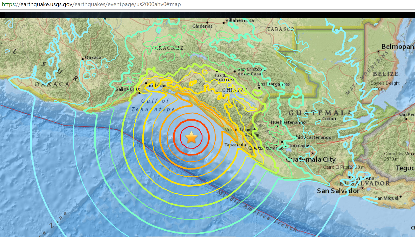
Overview figure of the region from Gavillot, et al., 2016. The box shows the location of our trip and the map shown below.

Overview of the field trip with the orange-red line showing most of our tracks and the yellow points my main obversation locations. I am using the GaiaGPS app for my mapping. It seems ok but I might look for a more geologically oriented app for the next trip.

Panorama and annotated overlay showing the major structures and bounded rock units

Pictures

View of the nice mountains (Dhaula Dhar Range) from the Kangra airport--a nice way to start the trip!

Katharina, Markus, and Rasmus with the impressive Dhaula Dhar Range behind as seen from the Kangra area.

Most of the group at a stop along the Main Boundary Thrust where a spring may indicate increased permeability along the fault zone (yellow-white material at left is travertine).

Upper Siwaliks at sunset

Katharina in the MCT mylonites.

Chambo Town--built on an important probably 10 ka terrace. We spent a pleasant cool night there.

Pretty agricultural terraces on a high terrace south of Chamba.

Nice terraces near the Chemera Reservoir.

Stair step terraces in a tributary a few km below the Chemera Reservoir.

Rasmus is a great teacher and it was wonderful to learn from him. Here he is near some fine grained schists discussing their reflection of the overall deformation in the MCT zone.

References cited
Dey, S., Thiede, R., Schildgen, T., Wittmann, H., Bookhagen, B., Scherler, D., and Strecker, M. Holocene internal shortening within northwest Sub-Himalaya: Out-of-sequence faulting of the Jwalamukhi Thrust, India: Tectonics, 2016a.

Dey, S., Thiede, R. C., Schildgen, T. F., Wittmann, H., Bookhagen, B., Scherler, D., … Strecker, M. R. (2016b). Climate-driven sediment aggradation and incision since the late Pleistocene in the NW Himalaya, India. Earth and Planetary Science Letters, 449, 321–331. https://doi.org/10.1016/j.epsl.2016.05.050

Gavillot, Y., Meigs, A., Yule, D., Heermance, R., Rittenour, T., Madugo, C., & Malik, M. (2016). Shortening rate and Holocene surface rupture on the Riasi fault system in the Kashmir Himalaya: Active thrusting within the Northwest Himalayan orogenic wedge. Bulletin of the Geological Society of America, 128(7), 1070–1094. https://doi.org/10.1130/B31281.1